Tag Archives: OSC

The CCD vs. CMOS Showdown: Why Monochrome Cameras Excel in Astrophotography Over One Shot Color

Introduction
One of the first things photographers must decide when venturing into astrophotography is what kind of camera sensor they’ll need to capture the beauty of the cosmos. Charge-Coupled Device (CCD) and Complementary Metal Oxide Semiconductor (CMOS) image sensors are two of the most common on the market (CMOS). Each has its own set of pros and cons that make it better or worse for astrophotography in certain situations. Further complicating matters is the ongoing discussion between advocates of monochrome and one-shot colour cameras.

Understanding CCD and CMOS Sensors
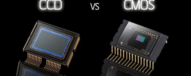
Light is converted into electronic signals by the CCD or CMOS sensor at the centre of a digital camera. The image quality, cost, and power consumption are all impacted, but in fundamentally different ways.

CCD Sensors
CCDs have been the go-to sensors for astronomy photography for quite some time. They are well-known for the exceptional clarity and sensitivity to light of their photographs. These sensors generate low-noise, high-quality images by transferring charge across the chip and converting it into voltage in a single spot: the array’s corner. In turn, this improves light collection by allowing for a greater pixel fill-factor. CCDs, on the other hand, are typically more costly and power-hungry than their CMOS counterparts. In addition, they experience ‘blooming,’ an effect in which overcharged pixels leak their energy into neighbouring ones.

CMOS Sensors
In contrast, CMOS sensors have shorter processing times and use less power because light is converted to voltage right at each pixel’s location. They have lower manufacturing costs, making them common in smartphones and consumer-grade cameras. Their read noise and sensitivity are typically higher than that of CCDs, though. Recently developed technologies have allowed CMOS sensors to catch up to and even surpass CCDs in terms of performance, closing the gap between the two.

Monochrome vs. One Shot Colour Cameras
After settling on a CCD or CMOS camera, the next big decision in astrophotography is whether to use a monochrome or one-shot colour camera.

One Shot Color Cameras
As the name implies, a One Shot Color camera takes a complete colour picture with just one click of the shutter. The Bayer mosaic used in these cameras covers each pixel with red, green, and blue filters. The greatest benefit of these cameras lies in their ease of use. Even amateur astronomers can easily take stunning, colourful pictures of the night sky with these instruments.

Monochrome Cameras
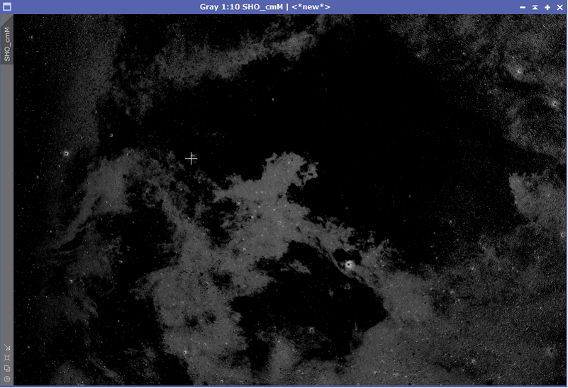
Images taken with a monochrome camera are grayscale. These cameras capture red, green, and blue light through individual filters and combine them into full colour in post-production. Even though using a monochrome camera is more difficult and time-consuming, there are some benefits.

Why Monochrome Cameras Excel in Astrophotography
In general, monochrome cameras have higher sensitivities than single-shot colour ones. They are up to three times as sensitive as cameras that use a Bayer filter because all of the light that reaches the sensor is used to create the image. This heightened sensitivities is especially helpful in low-light astrophotography.

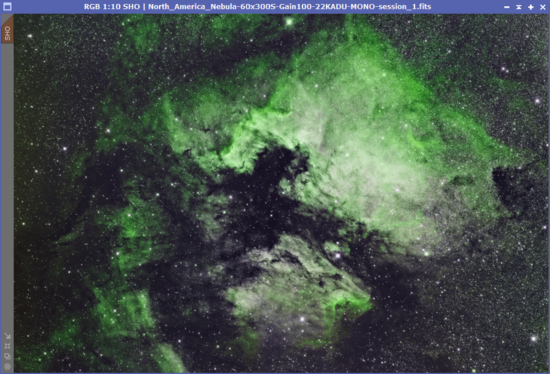
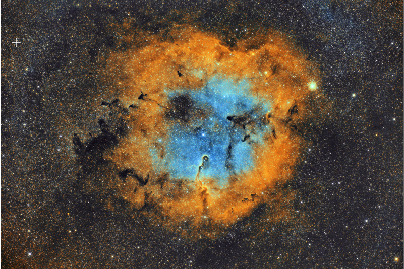
Additionally, more options and control can be had during the imaging process when separate filters are used with a monochrome camera. Using a hydrogen-alpha filter, astronomical photographers can isolate and emphasise specific wavelengths of light, such as the ionised hydrogen regions in nebulae. Imaging in light-polluted skies or capturing narrowband images greatly benefits from this ability.

Because the information for each colour channel is captured by the entire sensor rather than just a subset of pixels, as in one-shot colour cameras, the resulting images have greater resolution and detail.

Conclusion
In conclusion, CCD and CMOS sensors each have their uses in astrophotography, and the one you settle on will depend on your particular goals, financial constraints, and level of experience. Comparing monochrome and one-shot colour cameras, the former has better sensitivity, flexibility, and resolution while the latter is more user-friendly and saves time. Therefore, the investment in a monochrome camera and separate filters can be well worth it for serious astrophotographers seeking to capture the highest quality images.

Creating a Hubble Palette Image from OSC Dual Band Data

Many people like myself have transitioned from a MONO camera to a One Shot Colour (OSC) for whatever reason, for me it was all about not being able to get the required amount of time due to weather conditions here in the UK. When I first considered moving to an OSC camera, it dawned on me that I would not be able to produce the vibrant Hubble Palette images that I could produce by imaging with specific filters on my MONO camera, specifically Hydrogen Alpha (Ha), Oxygen 3 (OIII) and Sulphur Dioxide 2 (SII) which would then be mapped to the appropriate colour channels when creating the final image stack.

Now along came Dual and Tri band narrowband filters for OSC cameras which peaked my attention, the Dual Band filters allow Ha and OIII data to pass, the Tri Band filters allow Ha, Hb (Hydrogen Beta) and OIII to pass but at a high Nm value. I reached out to my friends at Optolong who had two filters, the L-eNhance and the L-eXtreme, the L-eNhance is a Tri Band filter, but after speaking with Optolong it would not work well for me at F2.8, so I went with the L-eXtreme Dual Band filter which has both the Ha and OIII at 7nm.

After receinving my ASI6200MC Pro, I decided to start acquiring data on a 1/2 to 2/3 moonlit nights on the North America Nebula, and so far when writing this post I had acquired a total of 60 frames of 300 seconds each at a gain value of 100, I processed the image my normal way in PixInsight and below is the result of the image:

North America Nebula, 60x300S at Gain100, Darks, Flats and BIAS frames applied with the ASI6200MC Pro using the Optolong L-eXtreme Dual Band 2″ Filter

I thought that my data looks good enough to work with and experiment with trying to build an SHO (Hubble Palette) image with, and I have spoken with Shawn Nielsen on this exact subject a few times so he gave me some hints and tips especially with the blending of the channels. So off I went to try and produce an SHO image.

Before we start, there are some requirements:

  • This tutorial uses PixInsight, I am not sure how you would acomplish this with Photoshop since I have not used PhotoShop for Astro Image Processing for a number of years
  • Data captured with a One Shot Color (OSC) camera using a Dual or Tri Band Narrowband filter
  • Image is non-linear…so fully processed

Step 1 – Split the Channels

In order to re-assign the channels, you have to split the normal image into Red, Green and Blue channels, I found this to work better on a fully processed “Non-Linear” image as above, once this was done, I renamed the images in PixInsight to “Ha” – Red Channel, “OIII” – Blue Channel and “SII” – Green Channel, this makes it easier for Pixelmath in PixInsight to work with the image names. Once this was done, I used PixelMath to create a new image stack with the channels assigned, and this is how PixelMath was configured

Red Channel = SII
Green Channel = 0.8*Ha + 0.2*OIII
Blue Channel = OIII

Once applied this produced the following image stack (do not close the Ha, OIII or SII images, you will need these later on):

SHO Combined image from PixelMath

Step 2 – Reduce Magenta saturation

As you can see from the above image, some of the brighter stars have a magenta hue around them, so to reduce this, I use the ColorMask plugin in PixInsight (You will need to download this), and selected Magenta

ColorMask tool with Magenta selected

When you click on OK, it will create the Magenta Mask which would look something like this:

Once the mask has been applied to the image, I then use Curves Transformation to reduce the saturation which will reduce the Magenta in the image


The result in reducing the magenta can be seen in this image, you will notice there is now no longer a hue around the brighter stars

Result after Magenta Saturation reduced using Magenta ColorMask and Curves Transformation

Step 4 – ColorMask – Green


Again using the Color Mask tool, I want to select the green channel, as we will want to manipulate most of the green here to red, so again ColorMask:

This then produced a mask that looks like the following:

Step 5 – Manipulate the Green Data

Once the Green Mask has been applied to the image, since most of the data in the image is green, we are looking to manipulate that data to turn it golden yellow, so for this we use the Curves Transformation again

The above Curves transformation was applied to the image three times whilst the the green mask was still im place, and this resulted in the following image changes:

Resulting image after green data manipulated in the red channel using Curves Transformation

So as you can see we are starting to see the vibrant colours associated with Hubble Palette images

Step 6 – Create a Starless version of the OIII Data

Now remember I said not to close out the separated channel images, this is because we are going to want ot bring out the blue in the image without affecting the stars, so for this we will turn the OIII image into a starless version by using the StarNet tool in PixInsight

Here’s the OIII Image before we apply StarNet star removal:

Default settings used in the StarNet process

This resulted in the following OIII image with no stars:

Step 7 – Range Selection on OIII Data

Because we do not want to affect the whole image, we will use the range selection tool on the starless OIII image to select areas we wish to manipulate, now we have to be careful that the changes we make are not too “Sharp” that they cause blotchy areas, so within the range selection tool, not only do we change the upper limit to suit the range we want to create the mask for, but we also need to change the fuzziness and smoothness settings to make it more blended, these are the setings I used:


Which resulted in the following range mask

Step 8 – Bring out the Blue with Curves Transformation

We apply the Range Mask to the SHO Image so that we can bring out the Blue in the section of the nebula where the OIII resides, with the range mask applied we will use the Curves Transformation Process again as follows:

Curves transformation process to increase blue, reduce red and increase saturation of image with rangemask applied

The result of which is:

Result after first curves transformation with RangeMask applied

As you can see we have started to bring out the blue data, but we are not quite there yet, with the range mask still applied, we will go again with the curves transformation only this time, just reducing the red element:


The result of the 2nd curves transformation with the Range Mask is as follows:

Resulting image after 2nd pass with Curves Transformation to remove the red elemtn in the range mask

Step 9 – Apply Saturation against a luminance mask

On the above image, we extract out the luminance and apply as a mask to the image, and we then use the Curves Transformation for the final time to boost the saturation to the luminance

Luminance Mask to be applied to image
Curves Transformation with Luminance Mask applied

Final Image

I repeated the same process on my Elephant’s Trunk Nebula that I acquired the data when testing out the ASI2400MC Pro and this was the resulting image:

I hope this tutorial helps in producing your SHO images from your OSC Narrowband images, I know many of my followers have been waiting for me to write this up, so enjoy and share.

ZWO ASI6200 62mpx Full Frame Camera Review

I recently wrote a review on the ZWO ASI2400 24mpx full frame camera, so I thought I would also do the same for the big brother which is the ZWO ASI6200 full frame camera with a mammoth 62mpx which I picked up from 365astronomy when returning the ASI2400 after the review. Looking at both of the cameras, there is no obvious difference from the outside except for the model number, both cameras are exactly the same size and feel roughly the same weight and the build quality is identicallyu exceptional.

ASI6200MC Pro One Shot Colour Camera

If we compare the specifications of the ASI6200 to the ASI2400 we can see where each camera has an advantage over the other:

ASI2400ASI6200
Weight700g700g
SensorIMX410IMX455
Sensor SizeFull FrameFull Frame
Pixel Size5.94um3.76um
Resolution24mpx62mpx
Full Well Capacity at 0 Gain100ke51ke
Qe>80%91%
ADC14-Bit16-Bit
High Gain Mode140100
Full well at High Gain Mode20ke18ke

So as you can see from the comparison on specification there are some differences, the ASI2400 has the edge on full well capacity, however the ASI6200 has a much more smaller pixel size as well as a higher Qe which to me gives the ASI6200 the edge over the ASI2400.

Now since both cameras are the exact same field of view due to them both being full frame sensors, the question is how does this affect resolution, clearly the ASI6200 has the upper hand having significantly more pixels than the ASI2400, but how does this translate to an image?

Iris Nebula taken with the ASI2400MC Pro, 82x150S at Gain 26, darks, flats and BIAS frames applied
Iris Nebula taken with the ASI6200MC Pro 48x150S at Gain 100, Darks, Flats and BIAS frames applied

As you can see, both cameras offer the exact same field of view, however when you zoom in on the images you start to see where the ASI6200 excels above the ASI2400 with the higher resolution

On the left is the ASI2400MC Pro and on the right is the ASI6200MC Pro

As you can clearly see from the above two images, the 6200 offers a much better resolution which will allow a much finer level of detail, however, depending on your sky conditions and focal length the ASI6200 might not be possible due to over or under sampling

You can see here, that on my SharpStar 15028HNT which has a Focal Length of 420mm the ASI2400 would lead to Under Sampling in my “OK” seeing conditions

But the ASI6200 shows in the green area:

If I increase the focal length to around 1150 the ASI6200 no longer becomes suitable and the ASI2400 is more suited to this focal length and sky conditions:

So as you can see, both the ASI2400 and ASI6200 is not a “One Size Fits All” scenario, you have to work out the best suitability depending on your conditions and equipment to be used.

From a price perspective, the ASI6200 is only slightly more expensive than the ASI2400, but both cameras offer the full frame capability and a fantastic field of view, but for me personally the ASI6200 beats the ASI2400 when using the focal length of my SharpStar 15028HNT. Just like it’s smaller version, the looks, feels, sounds and operates exactly the same way. Here is another image taken with the ASI6200 and then my Synthetic SHO version which I will be writing a tutorial on how to acomplish with Dual Band Filters.

North America Nebula – 60x300S at Gain 100 using the Optolong L-eXtreme Filter on the SharpStar 15028HNT
Synthetic SHO using the same data as the previous image

Either way, both ZWO cameras I have tested have been of awesome quality, and I would recommend either camera if you wish to go down the full frame route, but personally my favourite is the ASI6200MC Pro, more images to come since this is now my new camera.

QHY268C APS-C Colour Camera Review – Part 1

As many of you know, I have been using QHY cameras for a while, but with my plan to move to a RASA telescope next year and wanting to image with a bigger sensor than the QHY183M I decided to go for a bigger sensor but moving away from Mono, the latest addition to the QHY familly is the QHY268C Photographic Version. I had been talking to the QHY team for a long time about this particular camera, and finally I have one.

The QHY268C is a once shot colour camera based on the APS-C Sized back illimunated Sony IMX571 sensor, the camera has a true 16-Bit Analog to Digital Convertor (ADC), now there are a few camera models out there using this sensor, cameras such as the ZWO ASI2600, but one thing that sets the QHY268C apart from the others is the ability to have a 75ke full well capacity which is 25ke higher than the ZWO ASI2600. In my opinion, when imaging at fast focal ratios, a higher full well is desired to protect the colour around bright stars for example.

Opening the box I was greeted with a camera that was bigger and heavier than my 183M, but then the sensor is much bigger than the 183M anyway so this would be expected, but what I did not expect is the additional items that came with the camera:

Inside the box was:

  • QHY268C Photographic Version
  • UK mains plug for 12V AC adapter
  • 12V AC adapter
  • Car 12v power cable
  • Self locking power cable
  • 1.5M USB 3.0 cable
  • Dessicant drying tube
  • Self centering adapter plate
  • M54 to M48 adapter plate
  • M54 to 2″ nose adapter
  • A range of spacers to give you from 0.5mm to 13.5mm spacing
  • Associated screws for spacing adapters

QHY cameras have come along way since I bought my QHY183M, one of the things QHY has really worked on is amp glow, my early version of the QHY183M was renowned for was amp glow, which could be removed in image calibrations, but the QHY268C produces no amp glow whatsoever, below is a dark frame of 600S taken at -13.5C and you can clearly see there is no evidence of amp glow.

Single frame 600 seconds, Gain 26, Offset 30, -13.5C – Mono (Not Debayered)

Attaching to the telescope was pretty straight forward as I had already planned the imaging train before the camera arrived, since I will be using the SharpStar 15028HNT F2.8 Paraboloid Astrograph which has an M48 thread, I decided to keep the whole imaging train at M48 except for the camera of course which has an M54 thread, so I did not actually need to use any of the adapters that came with the camera, the reason for this is because I wanted to include a filter drawer, so my image train consists of the following (from telescope to camera)

  • TSOAG9 – TS Off Axis Guider (9mm)
  • TSOAG9-M48 – TS M48 Adapter for the OAG (2.5mm)
  • TSFSLM48 – TS 2″ Filter Drawer with M48 Thread (18mm)
  • M48AbstimmA05 – TS Optics 0.5mm Aluminium spacing ring (0.5mm)
  • TSM54a-m48i – TS M48 to M54 Adapter (1.5mm)
  • QHY268C with M54 Centering Adapter (23.5mm)

As you can see with all the above I reach my desired back focus of 55mm perfectly, if I was not going to be using a filter drawer (For my Optolong L-Pro and L-eXtreme filters), I would probably have stuck with the spacers that came with the camera. Below is a picture of the camera successfully connected to the telescope.

As far as settings go, after speaking with QHY on this at great length, I will be imaging in Mode 0 (Photographic mode) to avail of the massive 75ke full well, offset I will leave at 30, but Gain I will use two different settings, I will use Gain 0 for most bright objects with the L-Pro filter, but for the L-eXtreme, I’ll probably set a gain level of 26, luckily with SGPro I can set the gain level per object. From a cooling perspective I always image at -20C, one thing I have noticed is that this camera cools to exactly -35C below ambient, I tested this when the ambient temperature was 20.10 degrees, and the camera cooled down to -14.9C, it was always 25C lower until the ambient dropped below 15C and the camera remained at my setting of -20C.

The build quality of the camera is as expected having owned a QHY183M, one thing I did notice is that the fan in the QHY268C is much quieter than the 183M. Technical Details of the camera:

CameraQHY268CQHY183M
Image SensorSony IMX571Sony IMX183
Sensor SizeAPS-C1″
IlluminationBack IlluminatedBack Illuminated
Pixel Size3.76um2.4um
Effective Image26mpx20mpx
Full well capacity51ke
(75ke in extended mode)
15.5ke
ADC16-Bit12-Bit
Image Buffer Memory1GB/2GB128MB
Max Cooling Delta-35C-40C
Weight1006g650g

I can’t wait to get imaging with this camera, I have a very aggresive target list for this year in both RGB and Narrowband with the Optolong L-eXtreme filter, I will write part two of the review once I have some actual imaging data. Time to build my dark library.