Astrophotographers aiming to produce high-quality deep sky images rely on specialised software to stack and process their images. Two of the most popular choices for astronomical image stacking are PixInsight (PI) and Astro Pixel Processor (APP). While both tools offer powerful capabilities, they cater to different user needs and workflows. In this article, we explore the pros, cons, and key differences between PixInsight and Astro Pixel Processor to help you decide which is best for your astrophotography workflow.
PixInsight: Precision and Advanced Processing
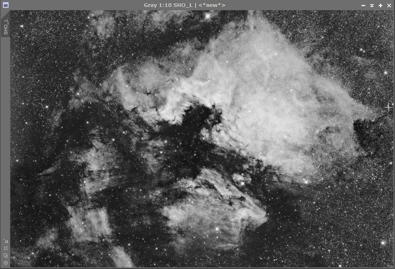
PixInsight has built a reputation as the gold standard for deep sky image processing, offering unparalleled control over stacking, calibration, and post-processing.
Pros of PixInsight:
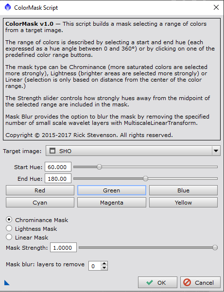
- Highly Customisable Processing – PI provides an extensive suite of tools and scripts that allow users to fine-tune every step of the image stacking and processing pipeline.
- Superior Calibration and Integration – The calibration and stacking tools in PI, such as Weighted Batch Preprocessing (WBPP), allow for precise control over light frames, darks, flats, and bias frames.
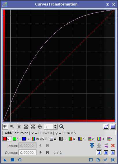
- Advanced Noise Reduction and Detail Enhancement – Features like Multiscale Linear Transform and Deconvolution provide powerful ways to refine details and suppress noise.
- Script and Process Automation – Users can automate complex workflows using PixelMath and scripting tools, streamlining repetitive tasks.
- Extensive Community Support and Plugins – A vast community of astrophotographers contributes to plugins, scripts, and detailed tutorials.
Cons of PixInsight:
- Steep Learning Curve – The interface is not beginner-friendly, requiring significant time and effort to master.
- No Native GPU Acceleration – PI relies heavily on CPU power, making processing times longer on large datasets compared to GPU-accelerated software. CUDA based GPUs can be added with the relevant runtime libraries.
- Expensive One-Time Purchase – The upfront cost can be high, though it does offer lifetime access without subscription fees.
- Recent Performance Issues on Windows (Reported by me) – Some users have reported significant performance issues with PixInsight on Windows 11, particularly with the latest 24H2 update. Discussions on the PixInsight forum indicate that versions 1.8.9-2, 1.8.9-3 and 1.9.2
exhibit degraded performance on certain high core CPU systems, which only appears to affect the Windows version of PixInsight. Users running high-end hardware may experience lower-than-expected processing speeds until a fix is released.
https://pixinsight.com/forum/index.php?threads/new-xeon-gen-5-system-low-performance-looks-like-1-8-9-2-3-dont-like-w11-24h2.24249/
Astro Pixel Processor: Simplicity and Efficiency
Astro Pixel Processor (APP) is designed for astrophotographers who want a more streamlined and intuitive approach to stacking and initial image processing.
Pros of Astro Pixel Processor:
- User-Friendly Interface – APP provides a more intuitive experience with a structured workflow, making it easier for beginners to get high-quality results.
- Automatic Calibration and Stacking – The software simplifies the pre-processing steps, requiring minimal manual intervention.
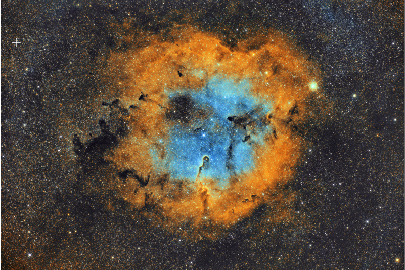
- Multi-Channel and Multi-Session Support – APP excels at handling mosaic projects and multi-filter data, making it ideal for narrowband imaging.
- Optimised for Speed – The use of efficient algorithms and multi-threading improves processing times, especially on modern CPUs.
- Excellent Gradient Reduction and Light Pollution Removal – The Local Normalisation Correction (LNC) and Adaptive Background Neutralisation (ABN) help correct background gradients effectively.
Cons of Astro Pixel Processor:
- Less Advanced Post-Processing – While APP is excellent for stacking, it lacks the sophisticated post-processing tools found in PixInsight.
- Subscription-Based Model – Unlike PI, APP requires an annual licence or a higher-cost perpetual licence.
- Limited Customisation of Algorithms – Users have less control over individual processing parameters compared to PixInsight.
Key Differences Between PixInsight and Astro Pixel Processor
| Feature | PixInsight (PI) | Astro Pixel Processor (APP) |
| Ease of Use | Steep learning curve, complex UI | User-friendly and intuitive |
| Stacking Power | Advanced, fine-tuned stacking | Fast, automated stacking |
| Calibration Tools | Extensive and manual control | Automated and efficient |
| Post-Processing | Industry-leading, full-featured | Basic adjustments available |
| Speed | CPU-based, can be slow, recent Windows issues reported | Faster due to optimised threading |
| Pricing | One-time purchase (£200+) | Subscription or perpetual licence (£100+/year) |
Which One Should You Choose?
- If you want maximum control, professional-level processing, and a comprehensive astrophotography workflow, PixInsight is the superior choice.
- If you prioritise ease of use, efficient stacking, and automation while still achieving excellent results, Astro Pixel Processor is a great alternative.
Many astrophotographers use both (Like me)—APP for stacking and initial processing, followed by PI for detailed refinement and final adjustments.
Regardless of your choice, both PixInsight and Astro Pixel Processor are powerful tools that can elevate your astrophotography, helping you extract the best possible detail from your hard-earned data.