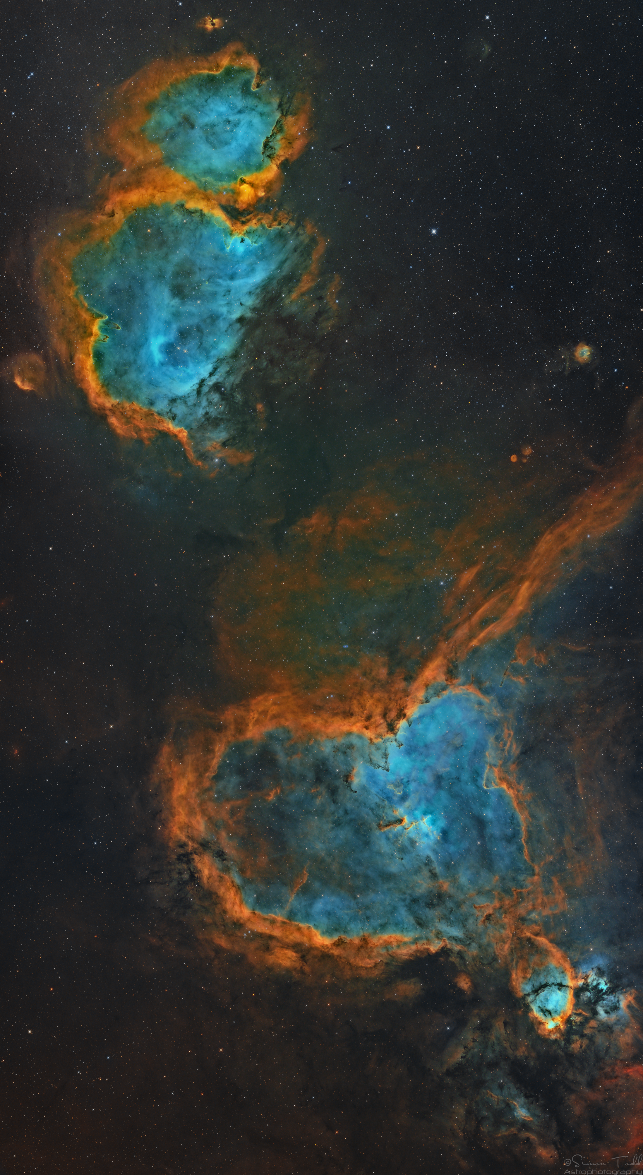
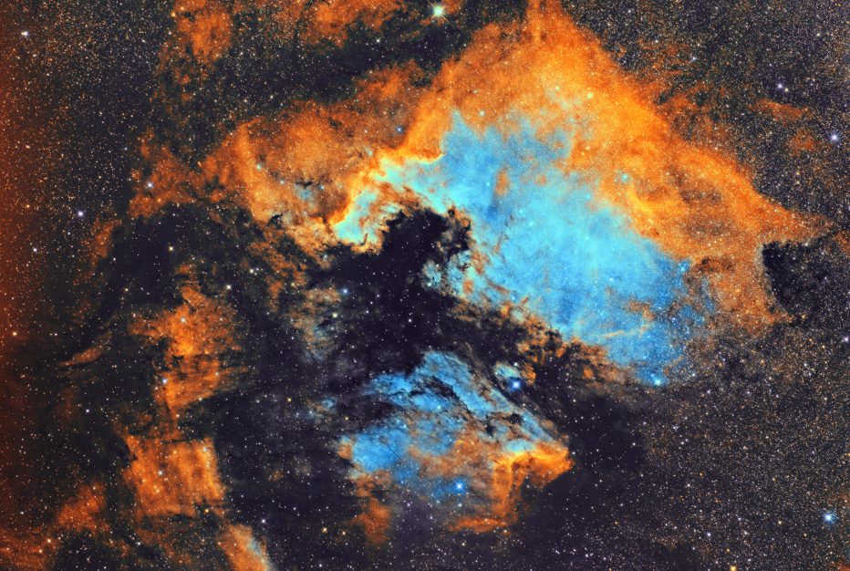
In the boundless theatre of the night sky, a spectacle of cosmic proportions gently unfolds. Here, through the unblinking eye of my camera, we witness the Heart and Soul Nebulae, celestial bodies of unimaginable scale and beauty. Captured in the vivid hues of the Hubble Palette, this image is the culmination of over 68 hours of patient vigil over the course of six months, a testament to the relentless march of time and space.
The Heart Nebula, known as IC 1805, and its companion, the Soul Nebula, IC 1848, are more than mere clusters of gas and dust. They are incubators of stars, cosmic nurseries where new celestial lives begin. Nestled within is the charmingly named Fish Head Nebula, a smaller star-forming region within this grand cosmic landscape.
Each pixel of this mosaic is a story, a tiny fragment of the universe’s narrative, captured through the artful blend of sulfur, hydrogen, and oxygen emissions. As we gaze upon this image, we are not merely observers but voyagers, embarking on an odyssey across the galaxy. It invites us to ponder our place in this magnificent universe, a reminder of both our insignificance and our profound connection to the cosmos.
In the grand scheme of things, this image is but a fleeting glimpse into the eternal dance of the cosmos. It is a humble offering to the beauty and complexity of the universe, a universe that continues to captivate and inspire us with its endless mysteries.
Catalog Names: IC 1805 (Heart Nebula) IC 1848 (Soul Nebula) Fish Head Nebula (Part of the Heart Nebula)
Acquisition Dates: 16 May 2023, 17 May 2023, 20 May 2023, 21 May 2023, 25 May 2023, 26 May 2023, 27 May 2023, 28 May 2023, 15 Jun 2023, 16 Jun 2023, 24 Jun 2023, 25 Jun 2023, 26 Jun 2023, 13 Jul 2023, 16 Jul 2023, 17 Jul 2023, 19 Jul 2023, 20 Jul 2023, 25 Jul 2023, 26 Jul 2023, 6 Aug 2023, 7 Aug 2023, 9 Aug 2023, 10 Aug 2023, 17 Aug 2023, 20 Aug 2023, 22 Aug 2023, 5 Sep 2023, 9 Sep 2023, 15 Sep 2023, 23 Sep 2023, 29 Sep 2023, 8 Oct 2023, 9 Oct 2023, 14 Oct 2023, 15 Oct 2023, 6 Nov 2023, 7 Nov 2023, 10 Nov 2023, 11 Nov 2023, 14 Nov 2023, 15 Nov 2023, 19 Nov 2023, 20 Nov 2023, 22 Nov 2023, 24 Nov 2023, 25 Nov 2023
Many people like myself have transitioned from a MONO camera to a One Shot Colour (OSC) for whatever reason, for me it was all about not being able to get the required amount of time due to weather conditions here in the UK. When I first considered moving to an OSC camera, it dawned on me that I would not be able to produce the vibrant Hubble Palette images that I could produce by imaging with specific filters on my MONO camera, specifically Hydrogen Alpha (Ha), Oxygen 3 (OIII) and Sulphur Dioxide 2 (SII) which would then be mapped to the appropriate colour channels when creating the final image stack.
Now along came Dual and Tri band narrowband filters for OSC cameras which peaked my attention, the Dual Band filters allow Ha and OIII data to pass, the Tri Band filters allow Ha, Hb (Hydrogen Beta) and OIII to pass but at a high Nm value. I reached out to my friends at Optolong who had two filters, the L-eNhance and the L-eXtreme, the L-eNhance is a Tri Band filter, but after speaking with Optolong it would not work well for me at F2.8, so I went with the L-eXtreme Dual Band filter which has both the Ha and OIII at 7nm.
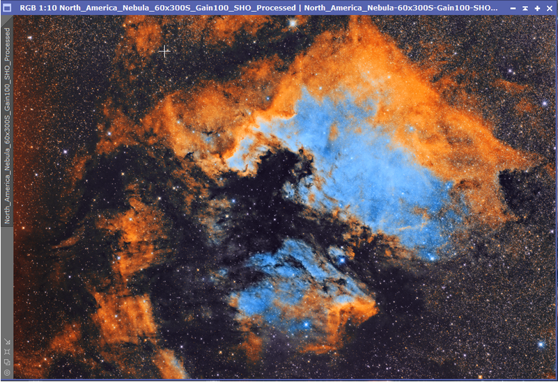
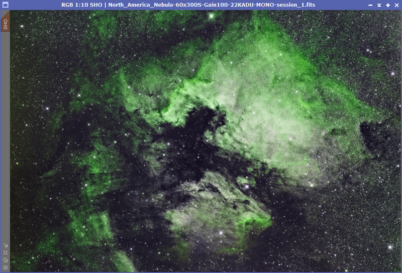
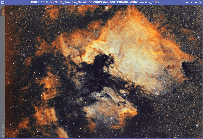
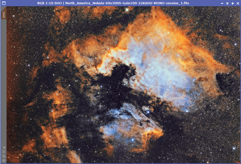
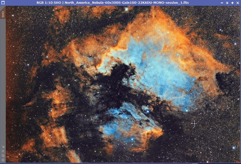
After receinving my ASI6200MC Pro, I decided to start acquiring data on a 1/2 to 2/3 moonlit nights on the North America Nebula, and so far when writing this post I had acquired a total of 60 frames of 300 seconds each at a gain value of 100, I processed the image my normal way in PixInsight and below is the result of the image:
North America Nebula, 60x300S at Gain100, Darks, Flats and BIAS frames applied with the ASI6200MC Pro using the Optolong L-eXtreme Dual Band 2″ Filter
I thought that my data looks good enough to work with and experiment with trying to build an SHO (Hubble Palette) image with, and I have spoken with Shawn Nielsen on this exact subject a few times so he gave me some hints and tips especially with the blending of the channels. So off I went to try and produce an SHO image.
Before we start, there are some requirements:
This tutorial uses PixInsight, I am not sure how you would acomplish this with Photoshop since I have not used PhotoShop for Astro Image Processing for a number of years
Data captured with a One Shot Color (OSC) camera using a Dual or Tri Band Narrowband filter
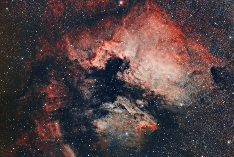
Image is non-linear…so fully processed
Step 1 – Split the Channels
In order to re-assign the channels, you have to split the normal image into Red, Green and Blue channels, I found this to work better on a fully processed “Non-Linear” image as above, once this was done, I renamed the images in PixInsight to “Ha” – Red Channel, “OIII” – Blue Channel and “SII” – Green Channel, this makes it easier for Pixelmath in PixInsight to work with the image names. Once this was done, I used PixelMath to create a new image stack with the channels assigned, and this is how PixelMath was configured
Red Channel = SII Green Channel = 0.8*Ha + 0.2*OIII Blue Channel = OIII
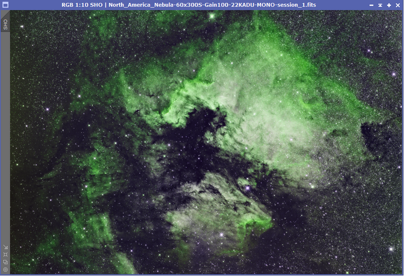
Once applied this produced the following image stack (do not close the Ha, OIII or SII images, you will need these later on):
SHO Combined image from PixelMath
Step 2 – Reduce Magenta saturation
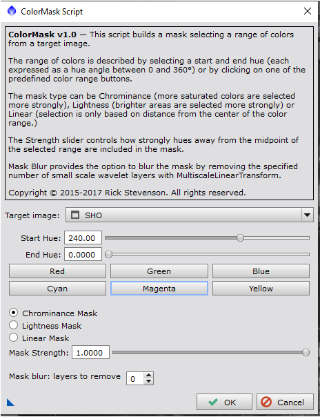
As you can see from the above image, some of the brighter stars have a magenta hue around them, so to reduce this, I use the ColorMask plugin in PixInsight (You will need to download this), and selected Magenta
ColorMask tool with Magenta selected
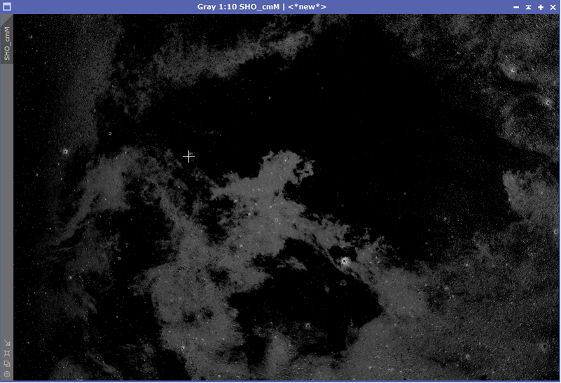
When you click on OK, it will create the Magenta Mask which would look something like this:
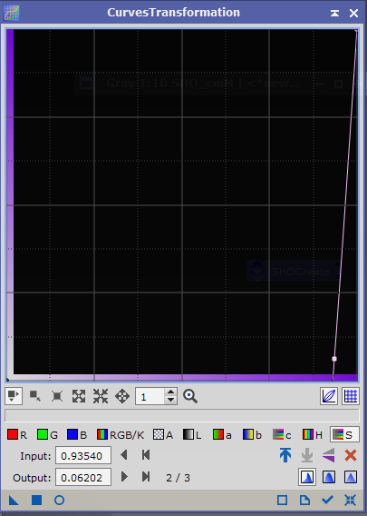
Once the mask has been applied to the image, I then use Curves Transformation to reduce the saturation which will reduce the Magenta in the image
The result in reducing the magenta can be seen in this image, you will notice there is now no longer a hue around the brighter stars
Result after Magenta Saturation reduced using Magenta ColorMask and Curves Transformation
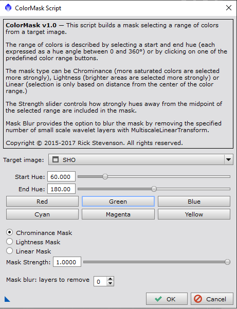
Step 4 – ColorMask – Green
Again using the Color Mask tool, I want to select the green channel, as we will want to manipulate most of the green here to red, so again ColorMask:
This then produced a mask that looks like the following:
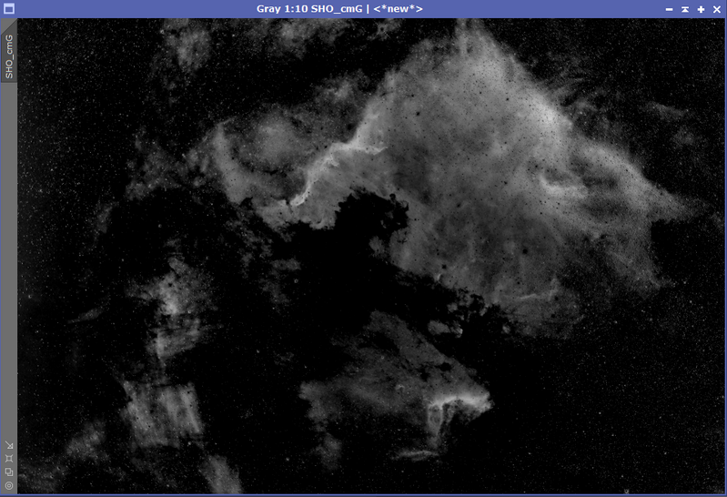
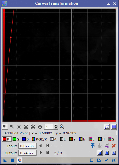
Step 5 – Manipulate the Green Data
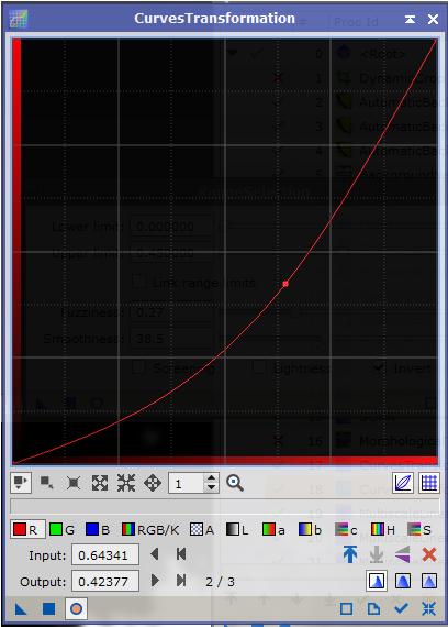
Once the Green Mask has been applied to the image, since most of the data in the image is green, we are looking to manipulate that data to turn it golden yellow, so for this we use the Curves Transformation again
The above Curves transformation was applied to the image three times whilst the the green mask was still im place, and this resulted in the following image changes:
Resulting image after green data manipulated in the red channel using Curves Transformation
So as you can see we are starting to see the vibrant colours associated with Hubble Palette images
Step 6 – Create a Starless version of the OIII Data
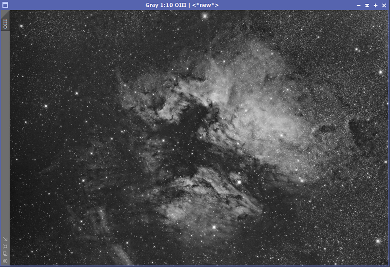
Now remember I said not to close out the separated channel images, this is because we are going to want ot bring out the blue in the image without affecting the stars, so for this we will turn the OIII image into a starless version by using the StarNet tool in PixInsight
Here’s the OIII Image before we apply StarNet star removal:
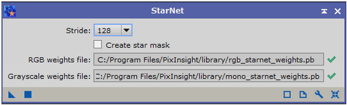
Default settings used in the StarNet process
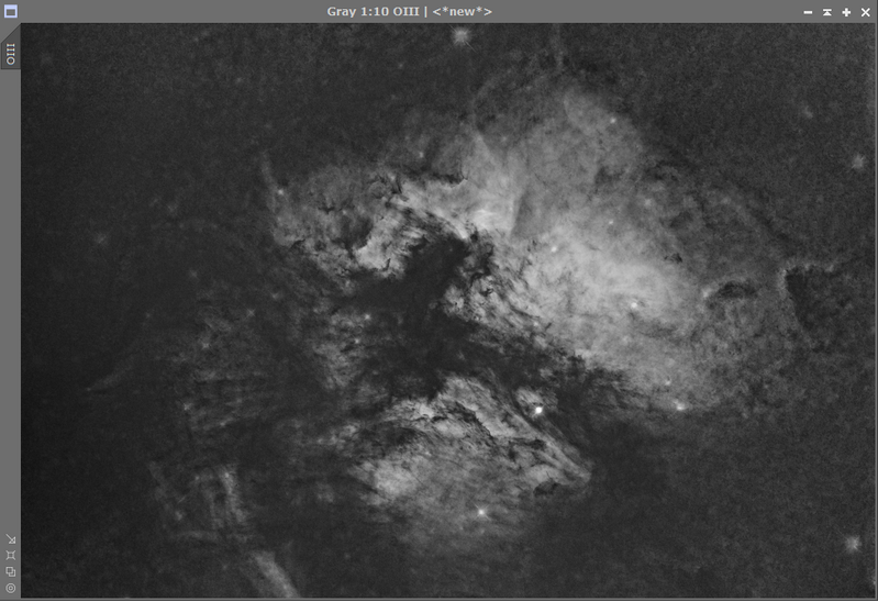
This resulted in the following OIII image with no stars:
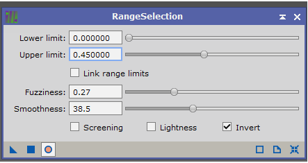
Step 7 – Range Selection on OIII Data
Because we do not want to affect the whole image, we will use the range selection tool on the starless OIII image to select areas we wish to manipulate, now we have to be careful that the changes we make are not too “Sharp” that they cause blotchy areas, so within the range selection tool, not only do we change the upper limit to suit the range we want to create the mask for, but we also need to change the fuzziness and smoothness settings to make it more blended, these are the setings I used:
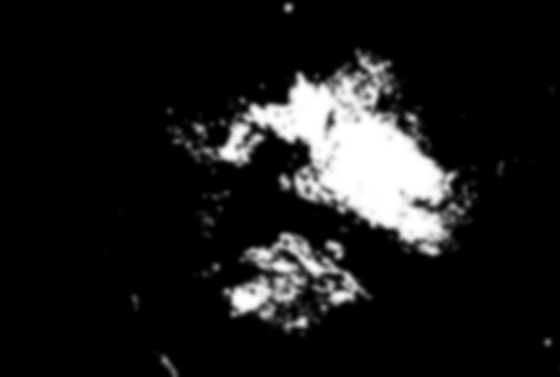
Which resulted in the following range mask
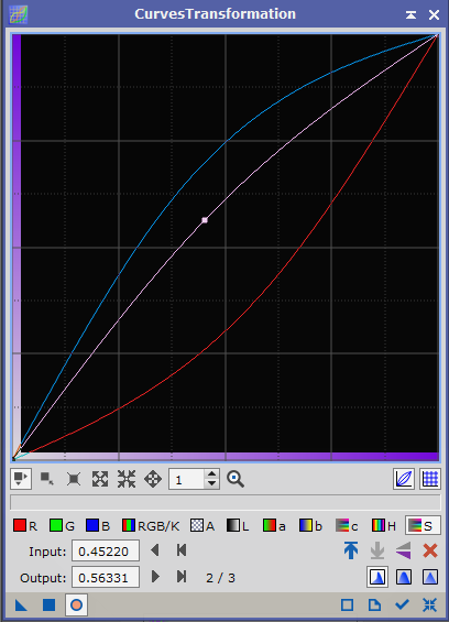
Step 8 – Bring out the Blue with Curves Transformation
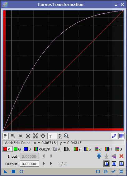
We apply the Range Mask to the SHO Image so that we can bring out the Blue in the section of the nebula where the OIII resides, with the range mask applied we will use the Curves Transformation Process again as follows:
Curves transformation process to increase blue, reduce red and increase saturation of image with rangemask applied
The result of which is:
Result after first curves transformation with RangeMask applied
As you can see we have started to bring out the blue data, but we are not quite there yet, with the range mask still applied, we will go again with the curves transformation only this time, just reducing the red element:
The result of the 2nd curves transformation with the Range Mask is as follows:
Resulting image after 2nd pass with Curves Transformation to remove the red elemtn in the range mask
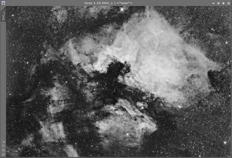
Step 9 – Apply Saturation against a luminance mask
On the above image, we extract out the luminance and apply as a mask to the image, and we then use the Curves Transformation for the final time to boost the saturation to the luminance
Luminance Mask to be applied to image
Curves Transformation with Luminance Mask applied
Final Image
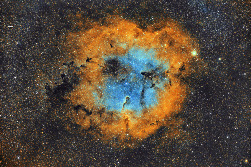
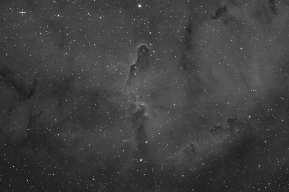
I repeated the same process on my Elephant’s Trunk Nebula that I acquired the data when testing out the ASI2400MC Pro and this was the resulting image:
I hope this tutorial helps in producing your SHO images from your OSC Narrowband images, I know many of my followers have been waiting for me to write this up, so enjoy and share.
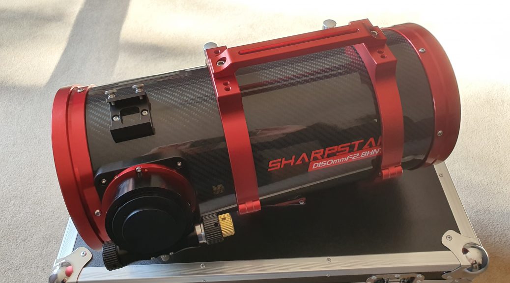
Having owned the Sharpstar 15028HNT, I decided I wanted a larger light bucket without really sacrificing on speed, so I opted for the big brother of the 15028HNT which is the SharpStar 20032PNT.
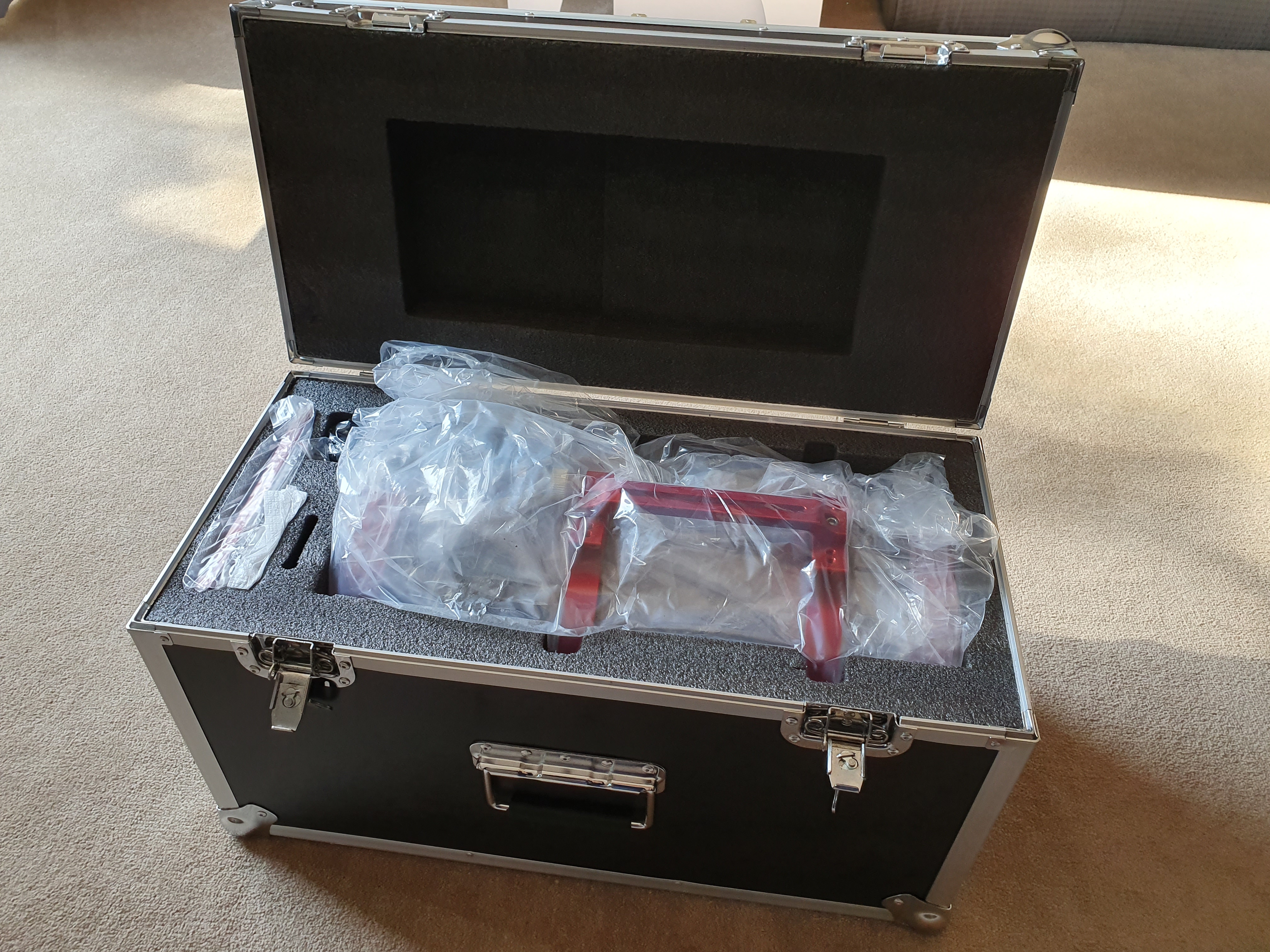
I picked up my 20032PNT from Zoltan at 365Astronomy, and could not wait to get it home and unbox it, so after removing it from not just one carboard box, but two, I was presented with a very large flight case, which evidently is a larger version than the one that came with the 15028HNT.
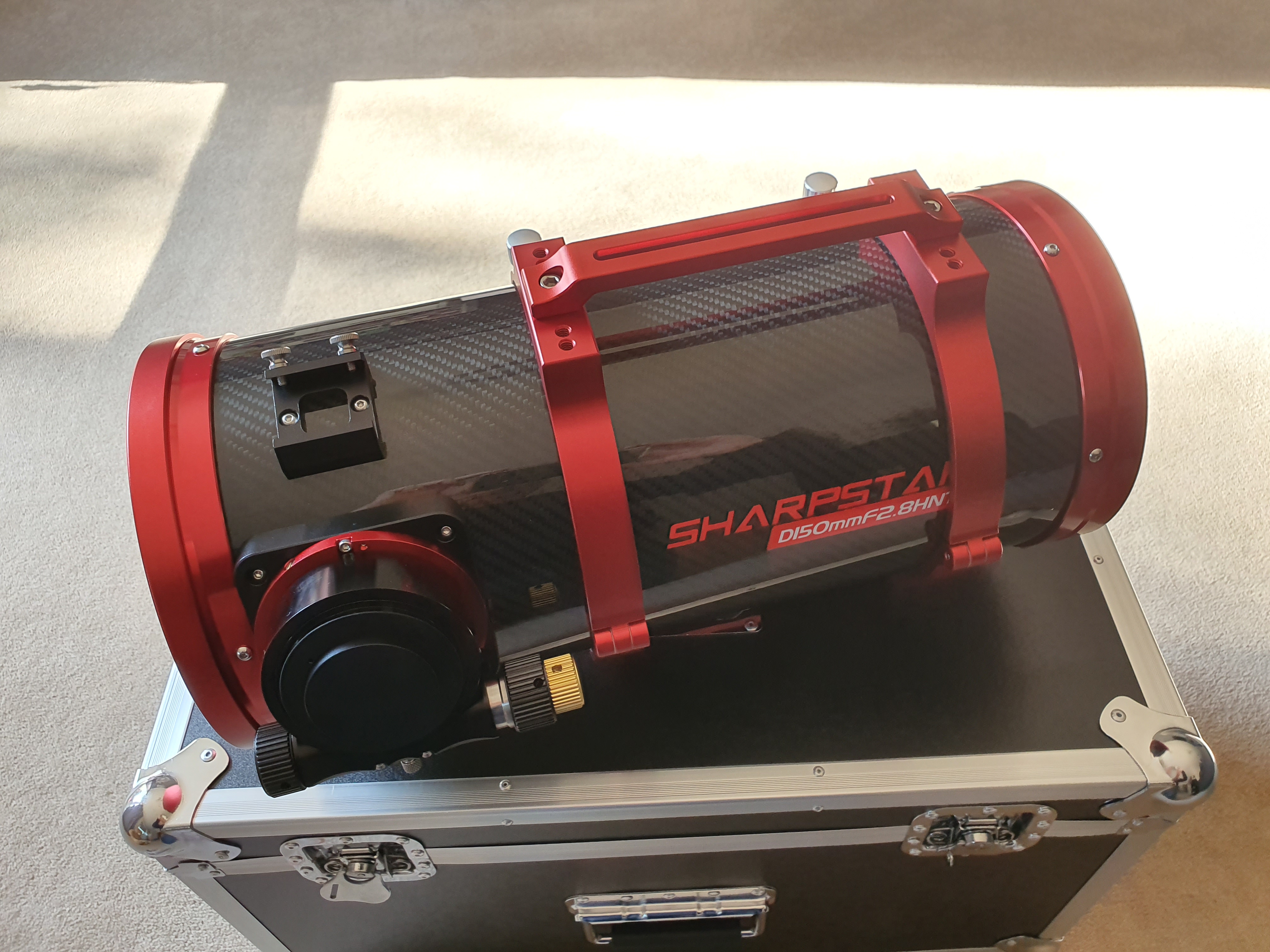
Once I had the scope unpacked and inspected everything, the first thing I noticed was the focuser, the 20032PNT has a large focuser, which is big enough to accomodate the reducer/corrector that has an M68 connector thread as well as an M54 and an M48 connector thread.
The scope is well built, as I would expect from the build quality of the 15028HNT, the red annodised alluminium tube rings just give that final touch of finese. The 3 inch focuser is very smooth, and will no doubt be able to handle quite a load of equipment.
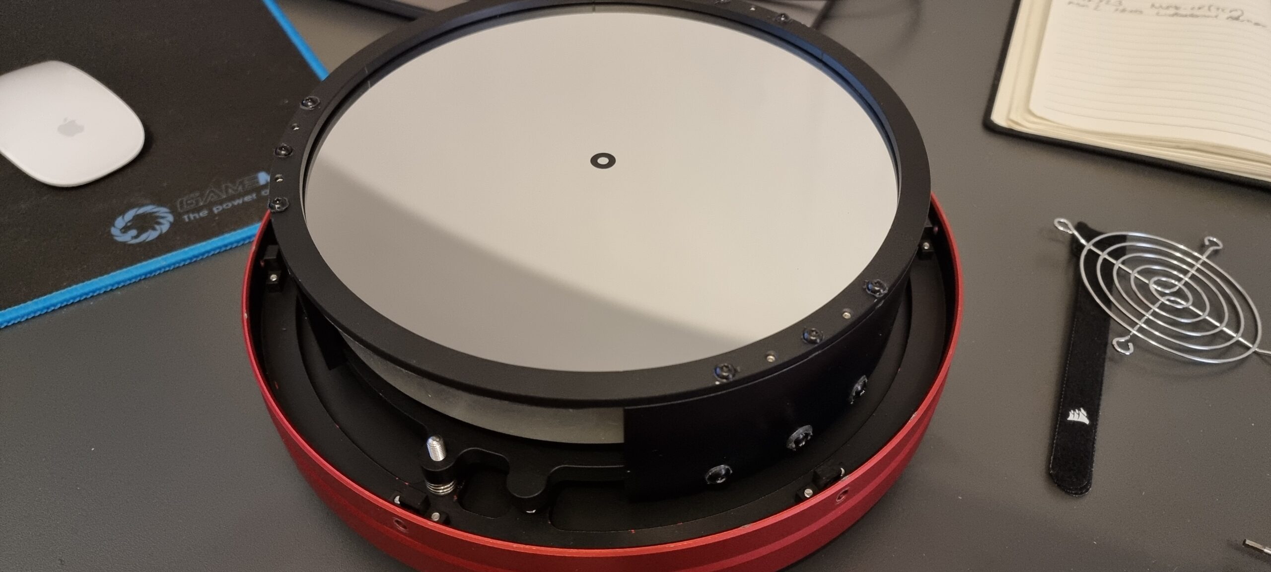
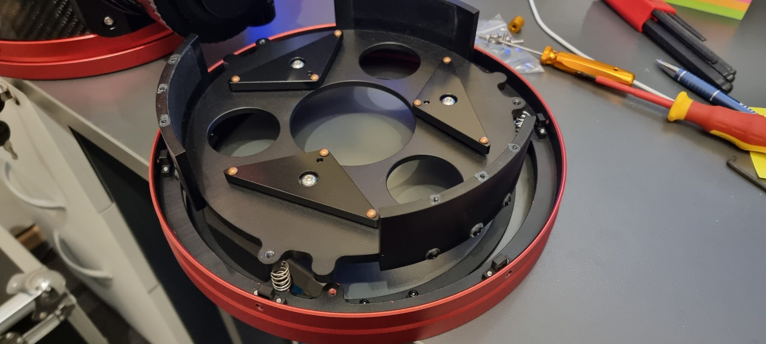
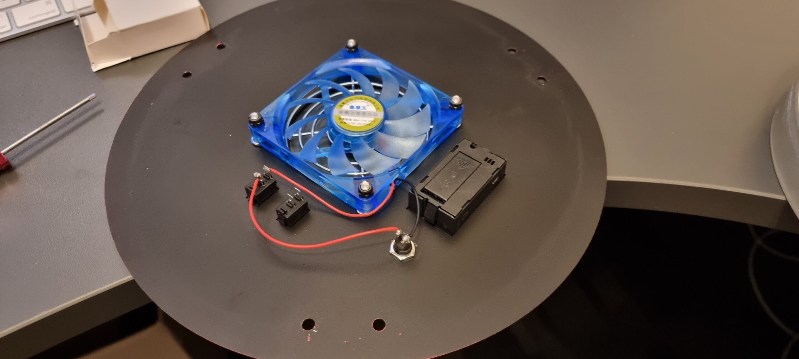
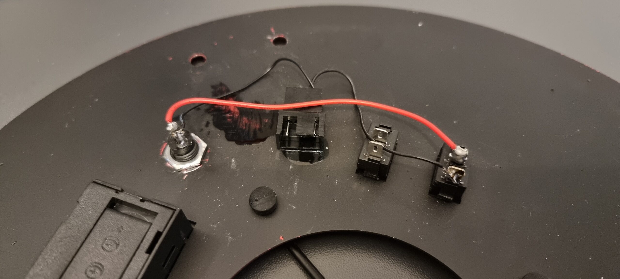
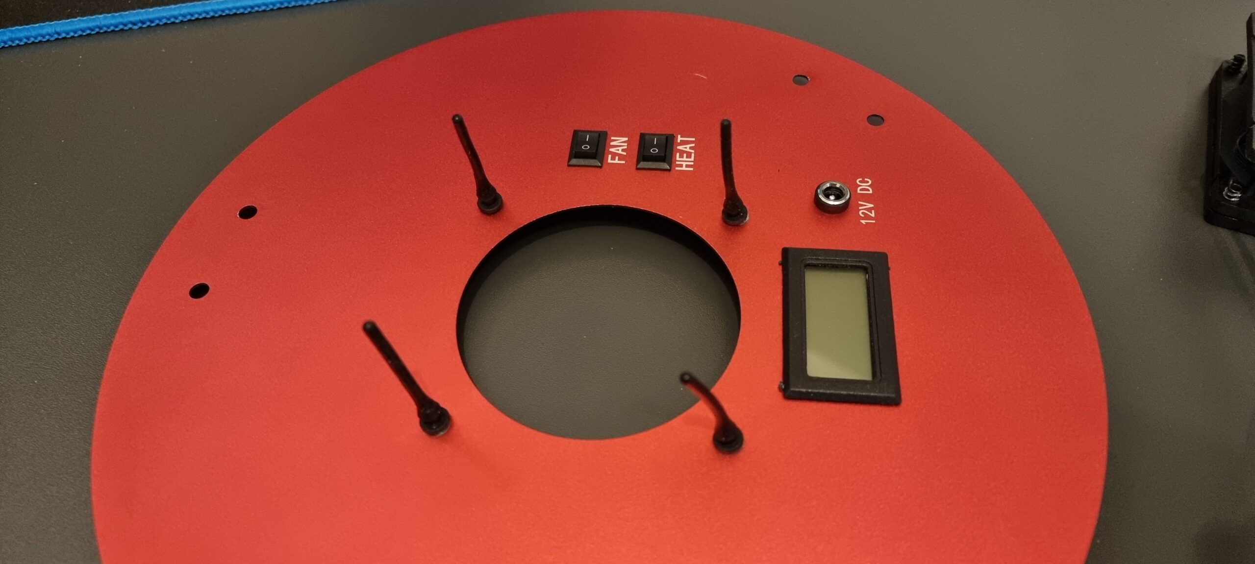
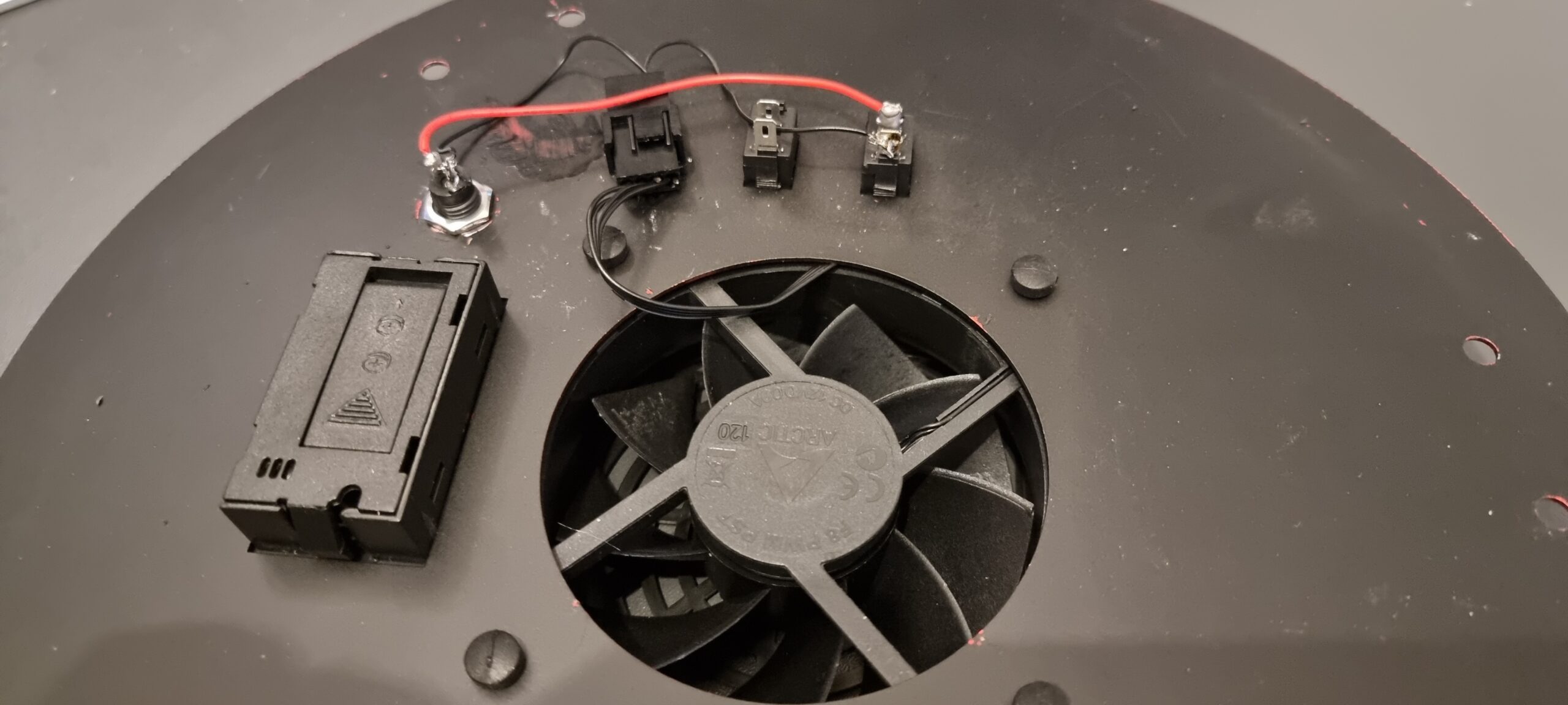
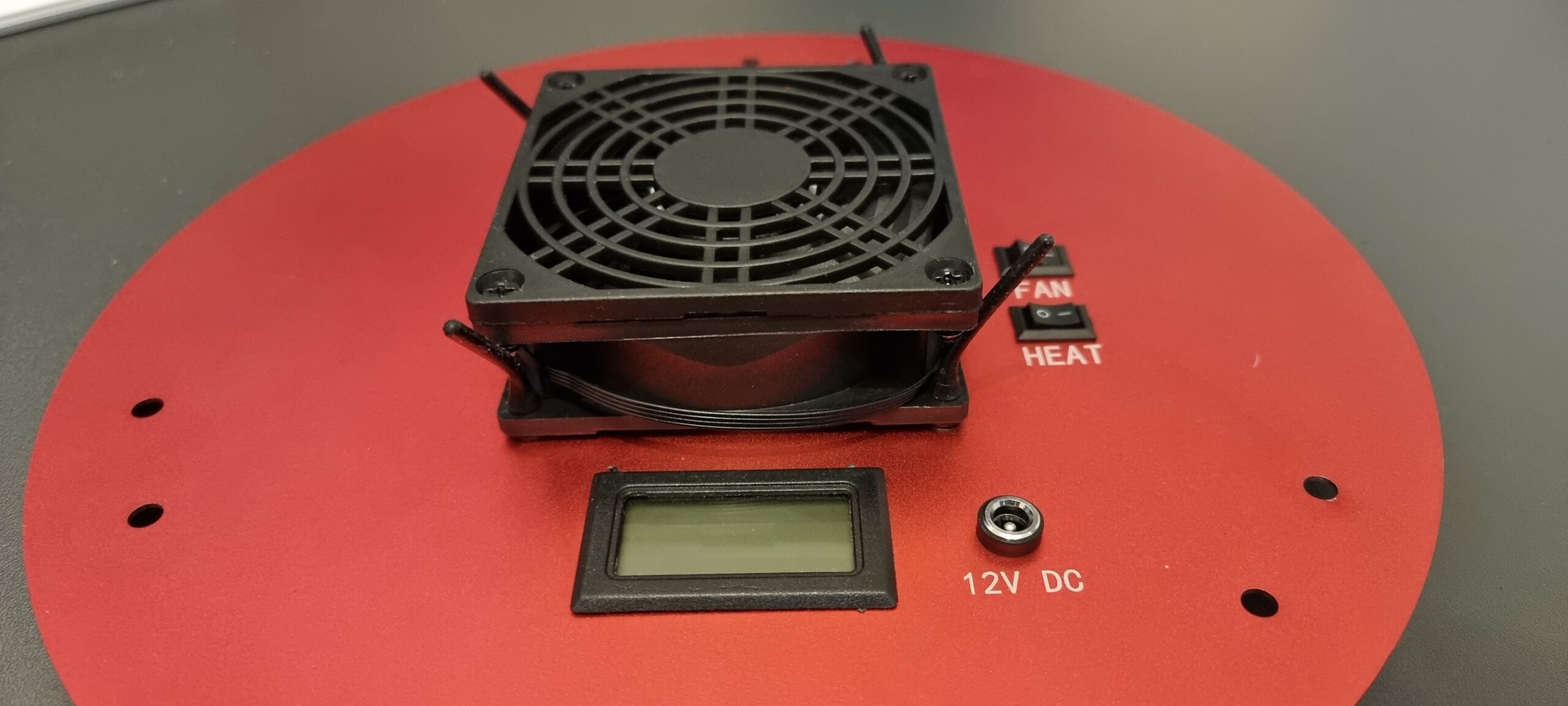
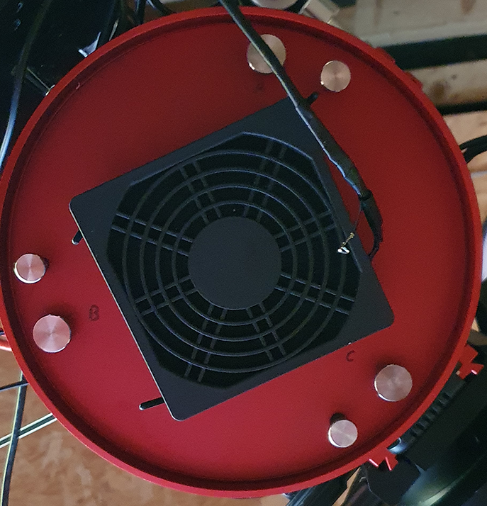
The first thing I planned to do was ensure that the primary mirror was secure and did not rock back and forward as well as replace the stock fan. I have fed back to SharpStar that they should mount the fan externally and also mount it with shock absorbing rubber mounters, and have the airflow into the tube from the back, rather than drawing air down the tube from the secondary. Here are my images of the fan replacement:
Primary Mirror assembly removed from OTAFan assembly with mirror removedStock FanStock fan removed and added in a PWM fan connector should the fan ever need to be replaced, it can be replaced without removing the mirror assemblyAnti vibration fan mounting pointsExternal fan connected to PWM connectorHow the fan looks from the outside, the image is missing the fan filter which I added afterwards
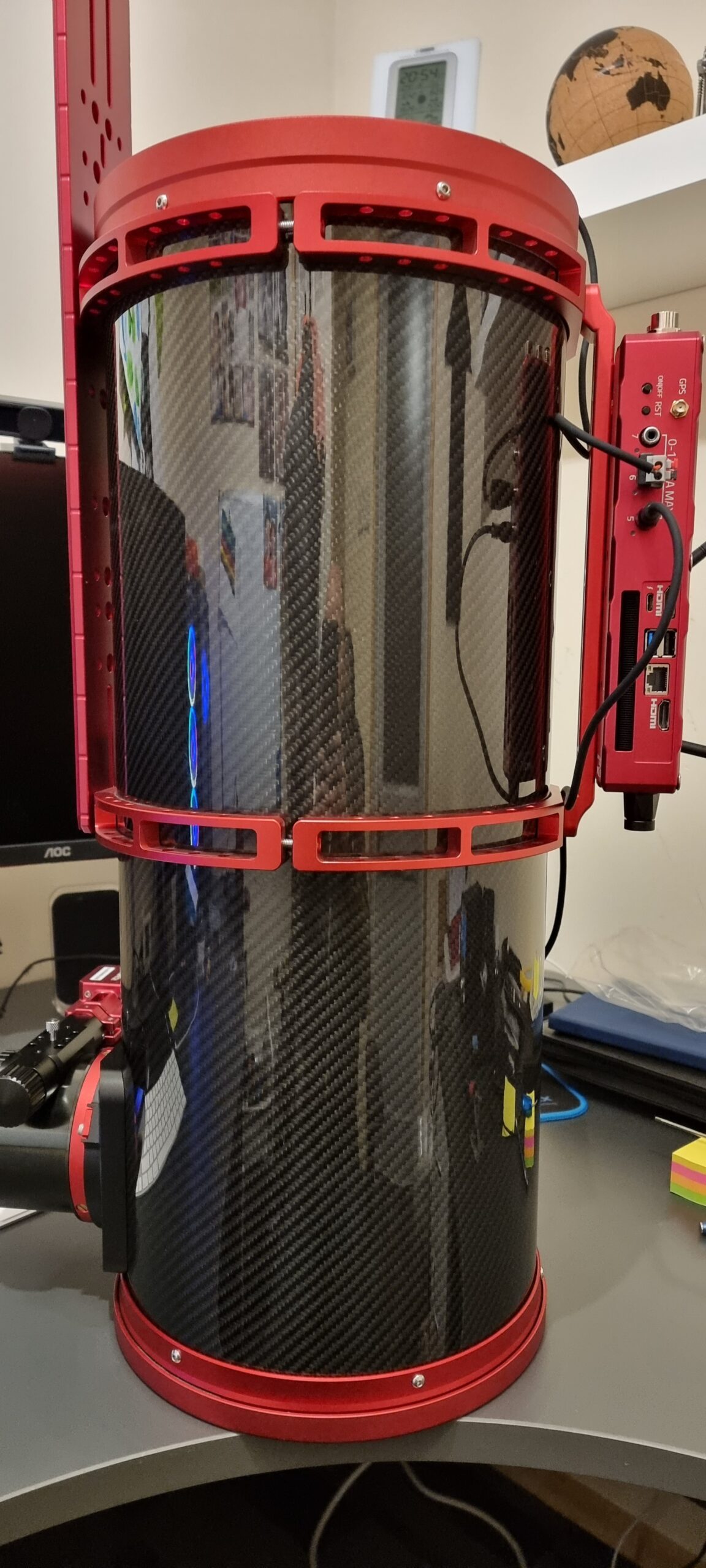
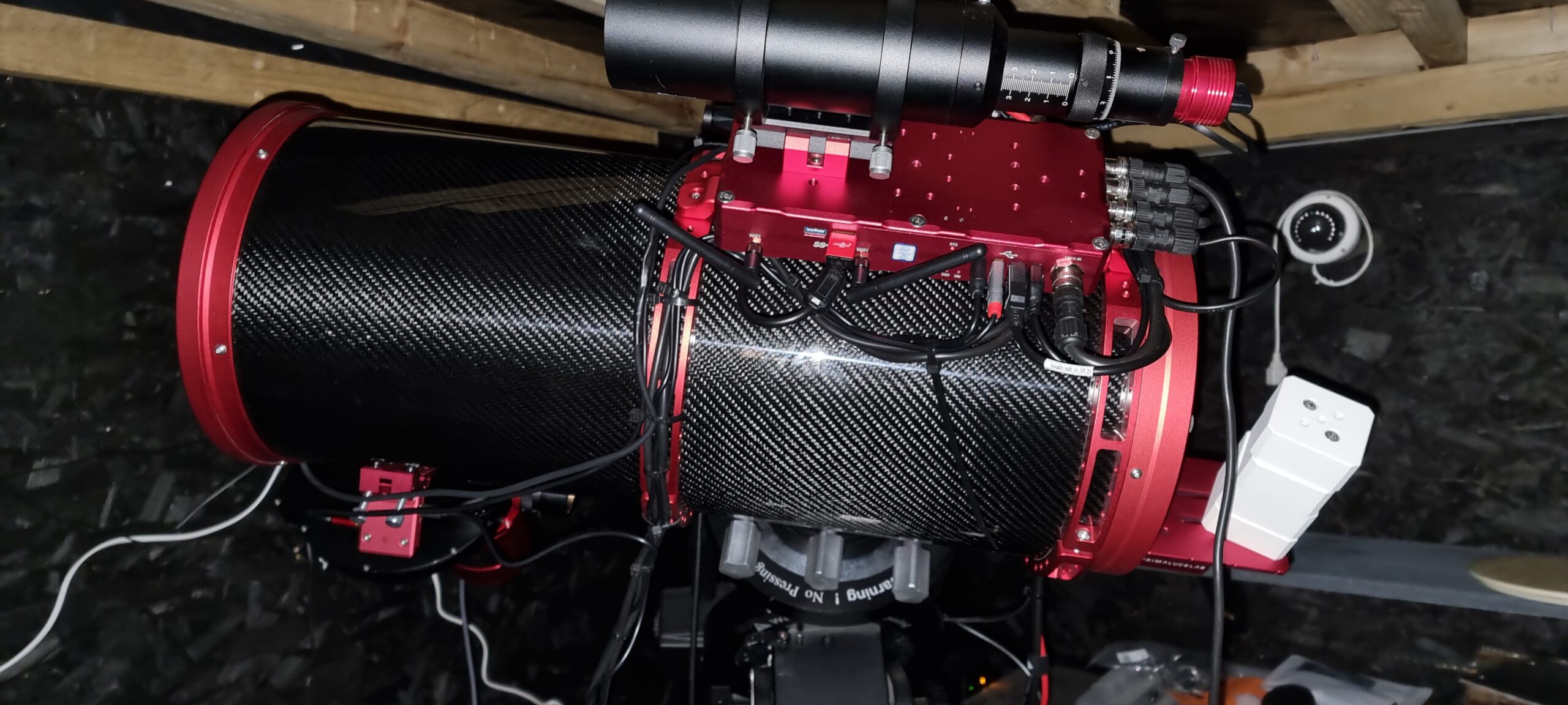
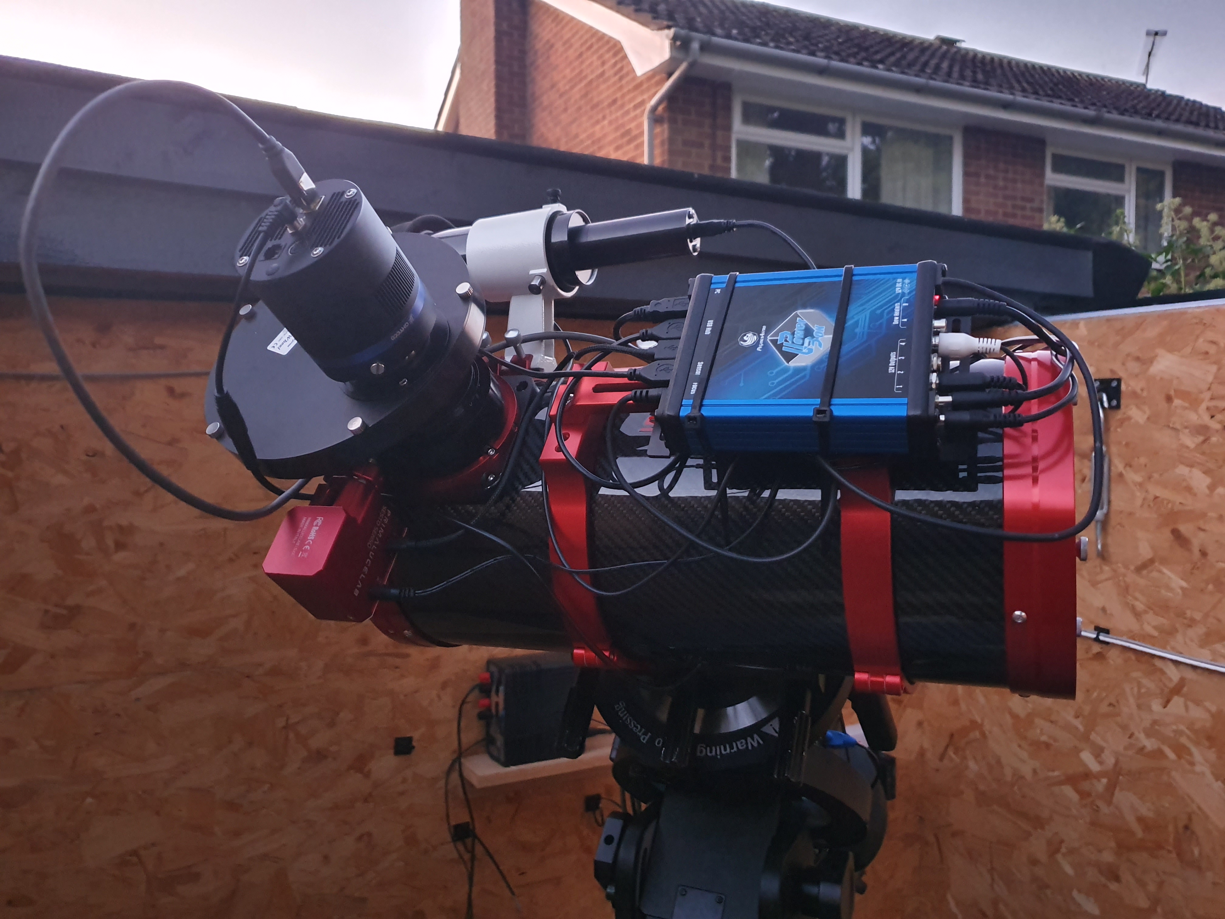
Once everything was back together, I mounted my Eagle4Pro onto the top bar, as well as added an extra long losmandy plate because I wanted the OTA as far forward as I could get it in order to have the camera in the right location without it hitting the mount at all.
And here is the scope on the mighty EQ8 Pro mount
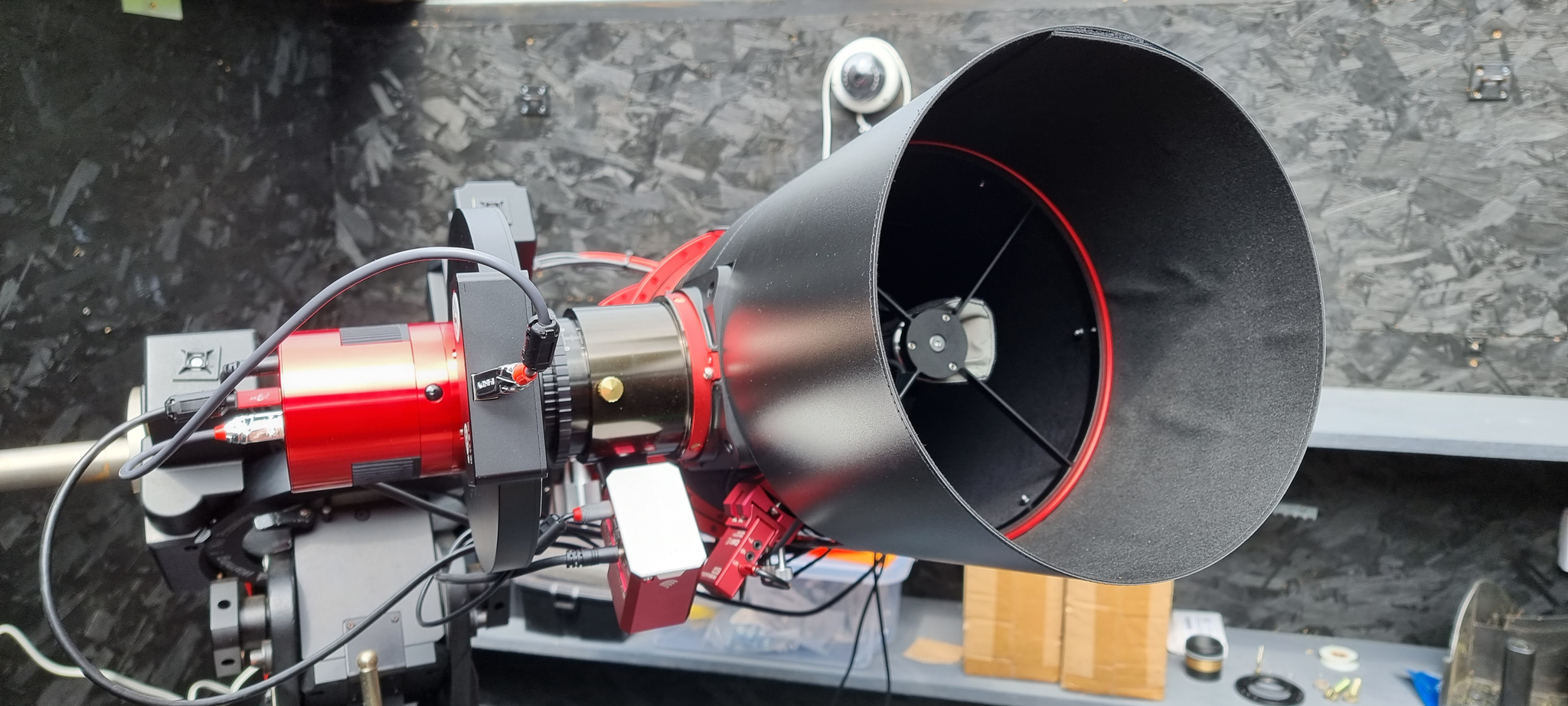
My first set of image testing did not go so well. My previous 15028HNT did not protrude above the walls of the observatory, so despite the fact that the secondary mirrors on both scopes are right up at the top of the tube, the 20032PNT was picking up stray light from my neighbour, so I had to adopt a dew shield that would extend the OTA by around 5 inches:
Scope with dew shield attached
Flats I first started to have issues with my flats that was taken with a flat panel, the flat frames would “Overcorrect” the images, but one thing I noticed that there was a lot of vignetting happening. Sky flats seemed to work better, but I was not happy with the vignetting. Now since I am using a full frame sensor on the ASI6200MM Pro, and the scope supports full frame, I was a little intrigued as to why I was getting so much vignetting, you can see from the master flat below that there was indeed a significant amount of vignetting.
Red Master Flat in PixInsight
I did some calculations and found what my problem was. Since my camera is full frame, it has a diameter of 44mm. The M54 connector on the telescope is 55mm away from the sensor, so a simple equation tells me that my light cone is larger than the M54 connector:
The internal diameter of the M54 connector is around 51mm, so the light cone was being restricted by around 10mm. So I had a custom M68 to M54 adapter made which is 28.5mm in length, the reason for this is because the backfocus from the M68 connector is 61mm, so if we apply our formula:
44 + (61/3.2) = 63.06mm, this is way below the internal diameter of the M68 connector male thread, so vignetting should be minimised. Now because I do have some M54 in my image train, I know I would not completely elliminate vignetting and this is why, using the above formula, we can work out the light cone at varying part of the imaging train:
12.5mm (EFW mating to camera) = 47.9mm 18mm (50.4mm Filters distance from sensor) = 49.62mm 32.5mm (Light entrance to EFW distance from sensor) = 54.15mm
As you can see, I should expect some vignetting to occur because the light cone at the EFW M54 connector (with around 51mm internal) is 54.15mm, so I would be clipping the light cone slightly, but the result is as follows, again red filter, you can see that the vignetting is significantly reduced:
Collimation was done using the exact same process I used on the 15028HNT, you can read the guide here.
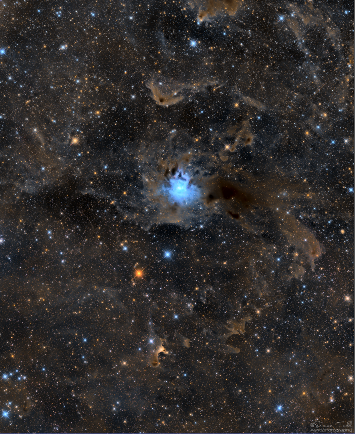
Conclusion: SharpStar have again produced an outstanding quality astrograph, with a massive focuser to take on the largest of imaging trains, as well as finishing off the product with high quality annodised OTA rings. I am extremely happy with the performance of the telescope, below is my first image which happens to be a 2 panel mosaic:
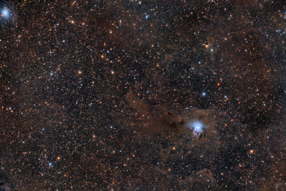
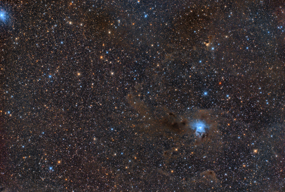
Iris Nebula, 2 Panel Mosaic, Each Panel consists of 151x60S frames at Gain100, for L, R, G and B, for the full resolution image please use this link
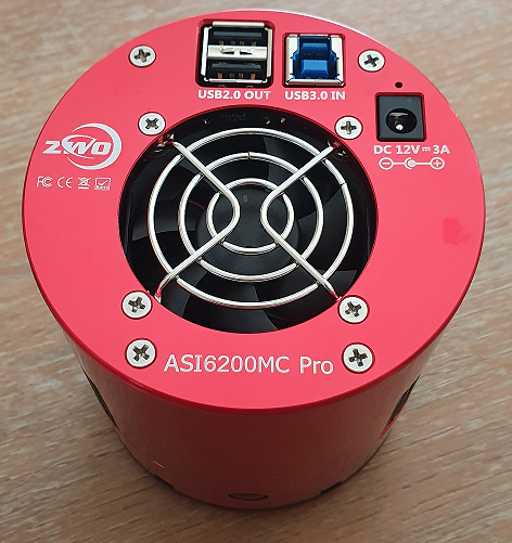
I recently wrote a review on the ZWO ASI2400 24mpx full frame camera, so I thought I would also do the same for the big brother which is the ZWO ASI6200 full frame camera with a mammoth 62mpx which I picked up from 365astronomy when returning the ASI2400 after the review. Looking at both of the cameras, there is no obvious difference from the outside except for the model number, both cameras are exactly the same size and feel roughly the same weight and the build quality is identicallyu exceptional.
ASI6200MC Pro One Shot Colour Camera
If we compare the specifications of the ASI6200 to the ASI2400 we can see where each camera has an advantage over the other:
ASI2400
ASI6200
Weight
700g
700g
Sensor
IMX410
IMX455
Sensor Size
Full Frame
Full Frame
Pixel Size
5.94um
3.76um
Resolution
24mpx
62mpx
Full Well Capacity at 0 Gain
100ke
51ke
Qe
>80%
91%
ADC
14-Bit
16-Bit
High Gain Mode
140
100
Full well at High Gain Mode
20ke
18ke
So as you can see from the comparison on specification there are some differences, the ASI2400 has the edge on full well capacity, however the ASI6200 has a much more smaller pixel size as well as a higher Qe which to me gives the ASI6200 the edge over the ASI2400.
Now since both cameras are the exact same field of view due to them both being full frame sensors, the question is how does this affect resolution, clearly the ASI6200 has the upper hand having significantly more pixels than the ASI2400, but how does this translate to an image?
Iris Nebula taken with the ASI2400MC Pro, 82x150S at Gain 26, darks, flats and BIAS frames appliedIris Nebula taken with the ASI6200MC Pro 48x150S at Gain 100, Darks, Flats and BIAS frames applied
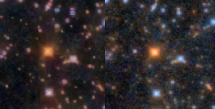
As you can see, both cameras offer the exact same field of view, however when you zoom in on the images you start to see where the ASI6200 excels above the ASI2400 with the higher resolution
On the left is the ASI2400MC Pro and on the right is the ASI6200MC Pro
As you can clearly see from the above two images, the 6200 offers a much better resolution which will allow a much finer level of detail, however, depending on your sky conditions and focal length the ASI6200 might not be possible due to over or under sampling
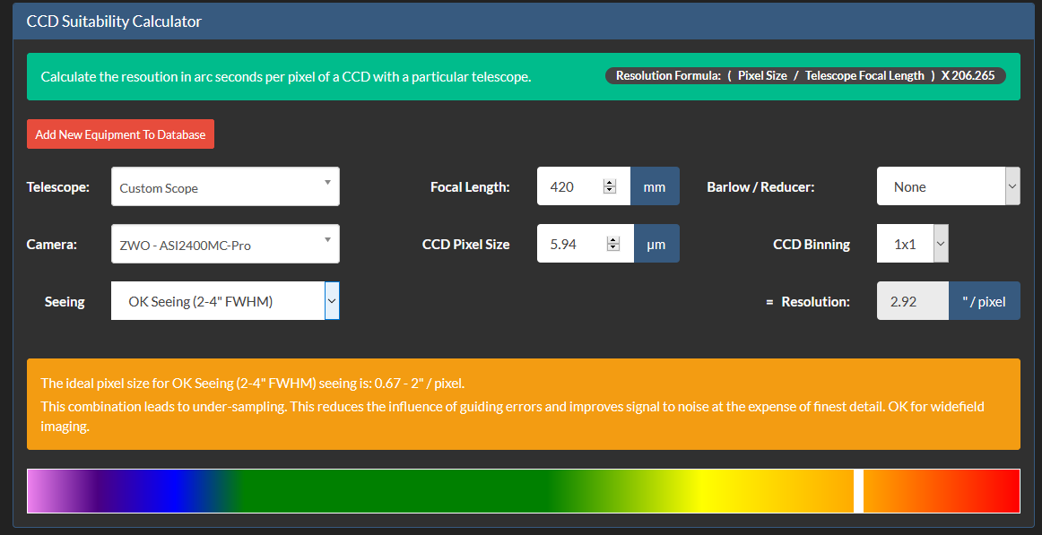
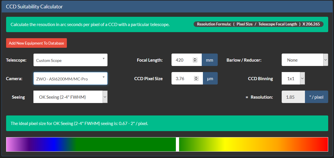
You can see here, that on my SharpStar 15028HNT which has a Focal Length of 420mm the ASI2400 would lead to Under Sampling in my “OK” seeing conditions
But the ASI6200 shows in the green area:
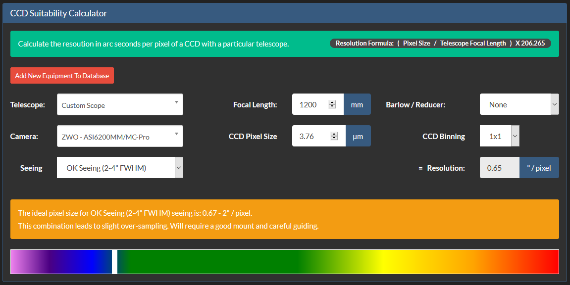
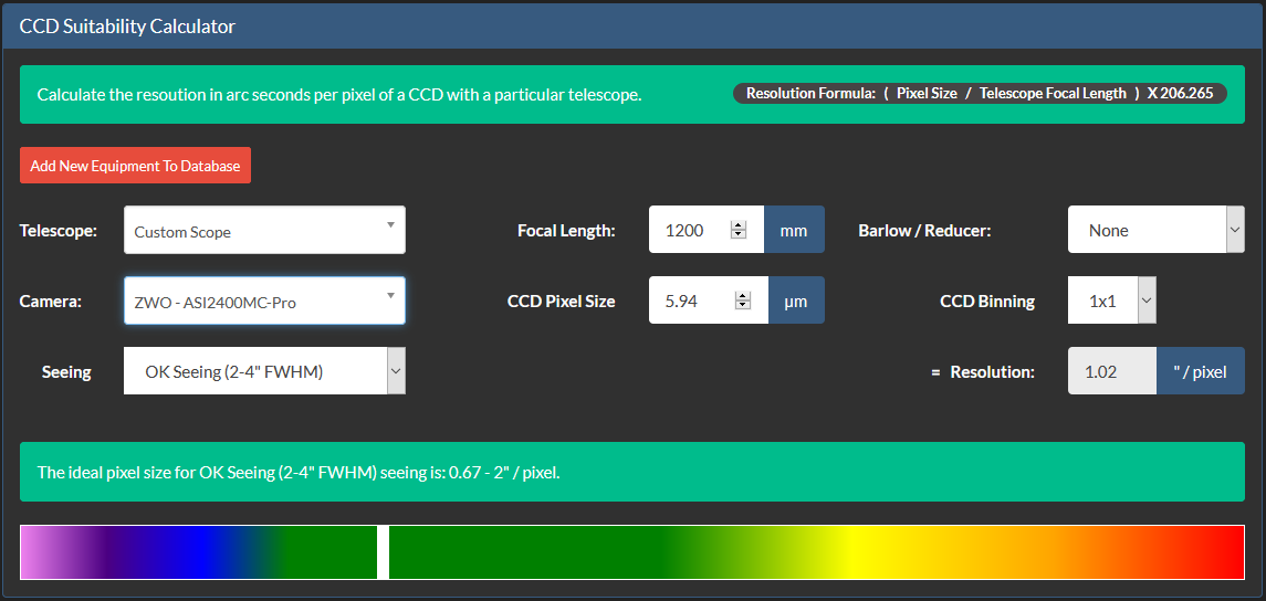
If I increase the focal length to around 1150 the ASI6200 no longer becomes suitable and the ASI2400 is more suited to this focal length and sky conditions:
So as you can see, both the ASI2400 and ASI6200 is not a “One Size Fits All” scenario, you have to work out the best suitability depending on your conditions and equipment to be used.
From a price perspective, the ASI6200 is only slightly more expensive than the ASI2400, but both cameras offer the full frame capability and a fantastic field of view, but for me personally the ASI6200 beats the ASI2400 when using the focal length of my SharpStar 15028HNT. Just like it’s smaller version, the looks, feels, sounds and operates exactly the same way. Here is another image taken with the ASI6200 and then my Synthetic SHO version which I will be writing a tutorial on how to acomplish with Dual Band Filters.
North America Nebula – 60x300S at Gain 100 using the Optolong L-eXtreme Filter on the SharpStar 15028HNTSynthetic SHO using the same data as the previous image
Either way, both ZWO cameras I have tested have been of awesome quality, and I would recommend either camera if you wish to go down the full frame route, but personally my favourite is the ASI6200MC Pro, more images to come since this is now my new camera.
If like me you own some sort of reflector telescope, whether this be a Newtonian, Dobsonian, Ritchey Chretien or as I have a Hyperboloid Astrograph then you’ll know that there is a very strong importance on collimation, the faster the optics the more critical collimation becomes, especially for imaging. After recently removing the rear mirror assembly for cleaning, as well as changing from the QHY183M to the QHY268C-PH amongst onther stuff in the imaging train, I wanted to share my experience and knowledge around collimation. Let’s start off with the details on what I use
Set of hex drivers (For adjusting the secondary mirror)
Part 1 – Aligning the Secondary Mirror with the Focuser
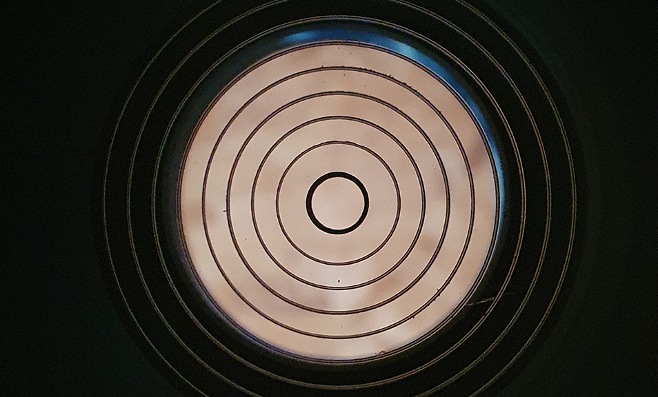
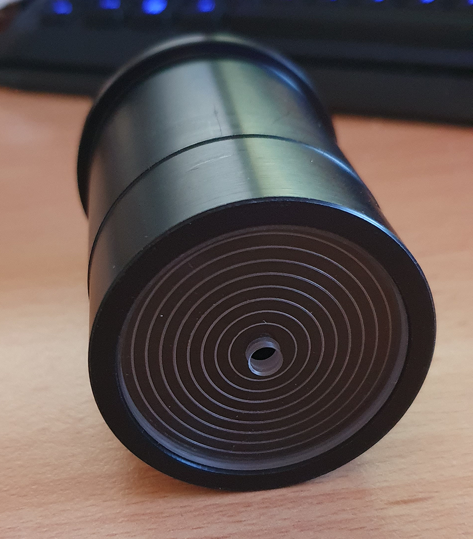
Now on my SharpStar 15028HNT, they recommend you unscrew and remove the corrector from the focuser, however I have found no difference in collimation with or without the corrector in place and because it is part of the optical train I’d rather include it in the collimation, so the first step for me since my primary mirror was currently removed was to check the secondary alignment with the focuser, as well as the rotation of the secondary in relation to the focuser, in order to do this, I use the Teleskop-Service Concenter eyepiece, the eyepiece itself has a set of rings engraved into the plastic apperture like so
Teleskop-Express Concenter Eyepiece markings on lower end of barrel
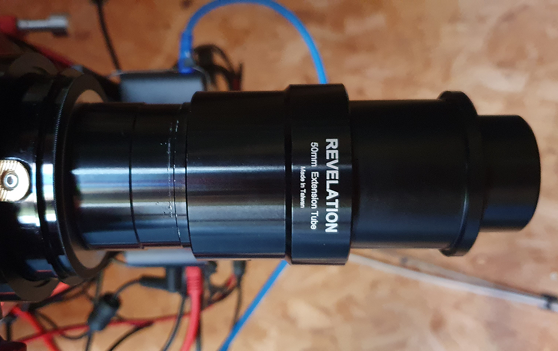
I ensure that my focuser is at the most inward position and since my SharpStar has an M48 thread on the focuser, I used a 2″ extension tube that has an M48 thread on it, and placed the concenter eyepiece in there:
M48 threaded 2″ Extension tube with Teleskop-Express Concenter Eyepiece
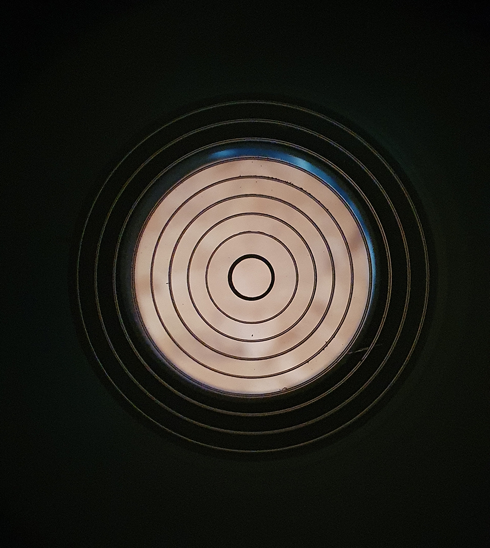
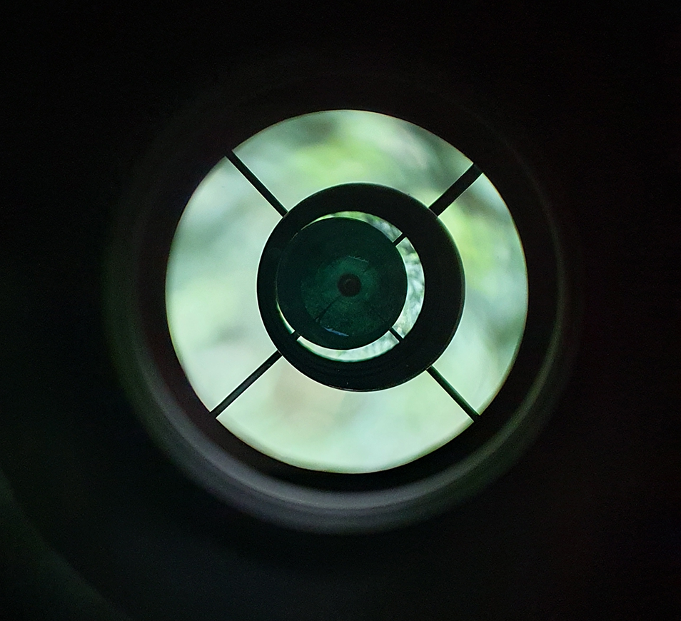
This serves well to get the rotation and alignment of the secondary with the focuser by ensuring that the mirror appears as a perfect circle between the rings, now you can adjust your focuser position in order to get the edge of the mirror to appear on the lines, this is what the view looks like through the concenter eyepiece:
Here you can see the secondary mirror appears circular and in line with the concenter eyepiece markings showing a successful alignment with the focuser
The blue at the top right of the image is a piece of card I stuck behind the secondary in order to show the edge of the mirror better.
As you can see my secondary mirror is pretty much perfectly aligned with the focuser and square with the focuser also, if your mirror shows up as more eliptical, this means the mirror needs to be rotated, if the mirror does not fit in within the circle itself, for example if it is over to the left or right, you will need to move the mirror forward or backwards by means of loosening or tightening the central screw that holds the secondary.
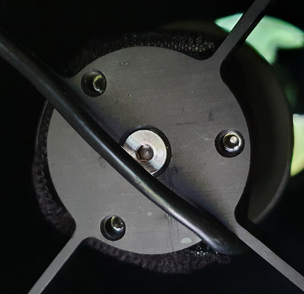
You can see from the following image, I have a central screw which is used for moving the mirror up or down the tube away from or closer to the primary, as well as rotation of the mirror, but then there is also the three collimation screws that are used to adjust the mirror direction itself which we will talk about in the next section
Here you can see the central adjustment screw for adjusting the mirror rotation and centering the mirror with the focuser, the three outer scres are used for adjusting the tilt of the mirror to align with the primary
Part 2 – Aligning the Secondary Mirror with Primary Mirror
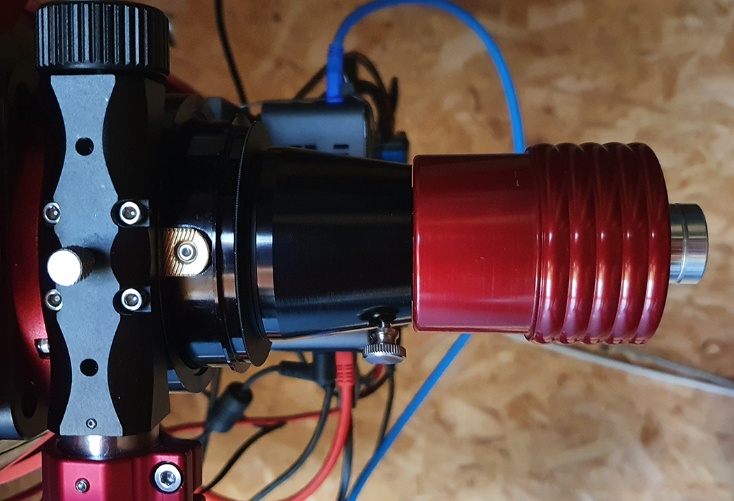
Now that we have our secondary mirror lined up and square with the focuser, the next step is to align the secondary with the primary, now for this I will use my FarPoint Astro Laser collimator, which itself has recently been collimated by FarPoint Astro, now you can re-use use the 2″ extension tube and place the laser into the tube, but for the SharpStar I will use the M48 to 1.25″ lockable adapter like so:
FarPoint Astro laser collmator in the SharpStar M48 to 1.25″ Adapter
Now the point of this part is to ensure that the laser hits the centre spot of the primary mirror, if it does not, then this is where you would adjust one or more of the three screws on the secondary, as you undo one, you should tighten the other two, as you can see from this image, I need not make any adjustments as the laser hits the centre of the primary perfectly:
Here you can see that the laser hits the primary mirror centre spot
Part 3 – Aligning the Primary Mirror
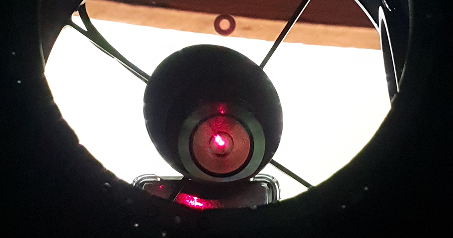
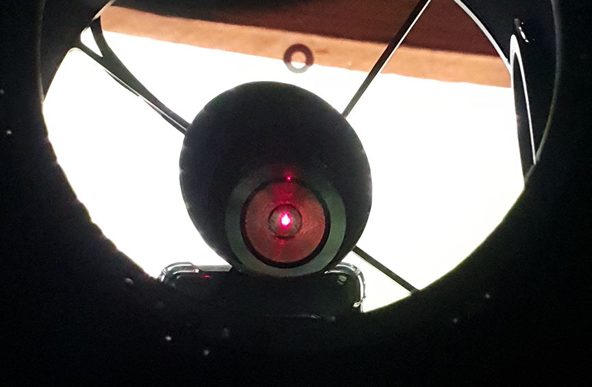
Now since I do not have to make any further adjustments to the secondary mirror, it is time to focus on the primary mirror, the trick here is to get the laser beam to return to the point of origin, here’s an example of the primary not being correctly aligned:
You can see two dots here, one is the laser aperture, the other is the reflection of the laser from the primary mirror, this reflection needs to meet the aperture
You can clearly see the red dot to the top left of the laser apperture, this means that the primary needs some adjustment by means of the three collimation screws which are situated on the rear of the primary mirror assembly:
Here you can see the primary mirror collimation screws, the larger push/pull the mirror, the smaller are locking screws to secure the mirror in place after successfully collimating.
Most telescopes have a push – pull method here, turning anti-clockwise will push the mirror further up the tube, whereas turning clockwise will pull the mirror towards the bottom of the tube, it is very important not to keep turning anti-clockwise because this could result in the screws becoming disconnected from the primary mirror. After an adjustment on a couple of the collimation screws, my primary is now aligned properly as the laser beam returns into the laser apperture:
Here you can see that there is no additional dot, the dot is centered right on the laser aperture indicating primary alignment is complete
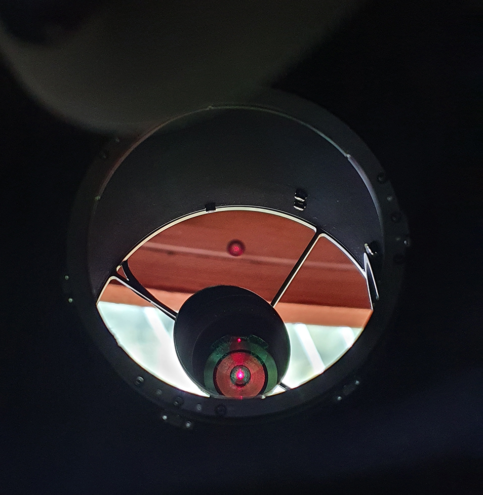
Once the laser collimation has been completed, it is easy to verify this with the FarPoint Auto-Collimator, the eyepiece has a mirror inside which allows you to see where the centre spot of the mirror is and will form a slightly pale dot in the middle, if the dot appears in the middle then you have your collimation pretty much spot on after following the above, maybe a very slight adjustment on the primary collmation screws is all that is required, you can see here what the view looks like:
It is also normal on faster telescopes to see the mirror appearing offset as opposed to central to the OTA itself. Once completed, I would typically then perform a star field test and I prefer to use the Multi Star Collimation in CCD Inspector for this, you can of course use the de-focused star method.
I hope you found this useful, I just thought I would share my process in performing collmation to help others who may be on that journey also.
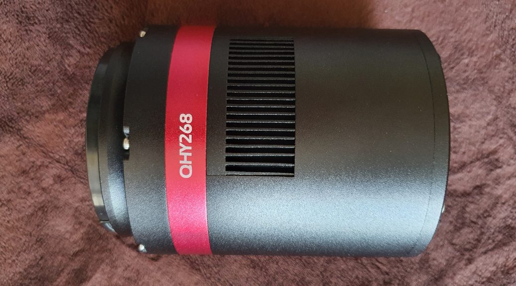
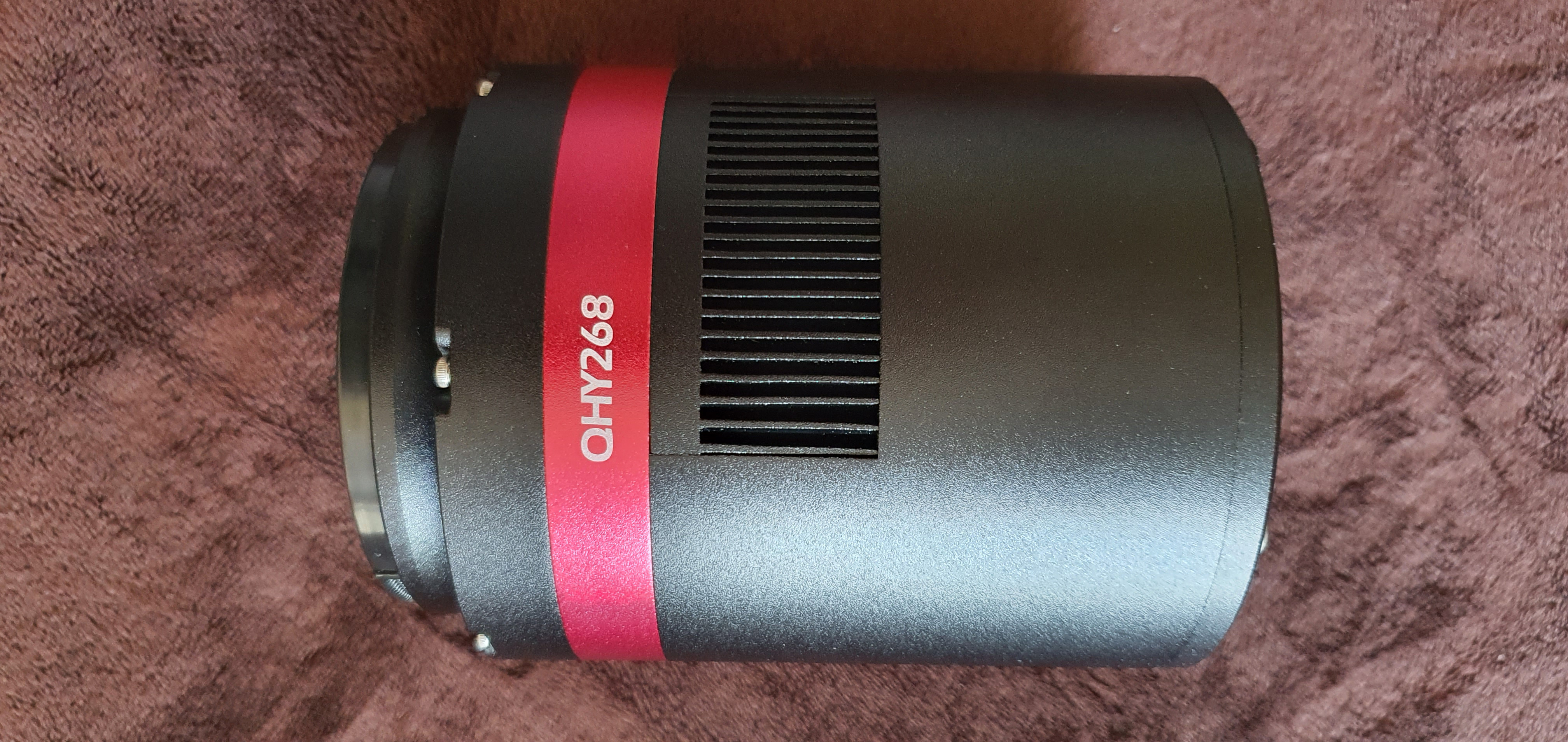
As many of you know, I have been using QHY cameras for a while, but with my plan to move to a RASA telescope next year and wanting to image with a bigger sensor than the QHY183M I decided to go for a bigger sensor but moving away from Mono, the latest addition to the QHY familly is the QHY268C Photographic Version. I had been talking to the QHY team for a long time about this particular camera, and finally I have one.
The QHY268C is a once shot colour camera based on the APS-C Sized back illimunated Sony IMX571 sensor, the camera has a true 16-Bit Analog to Digital Convertor (ADC), now there are a few camera models out there using this sensor, cameras such as the ZWO ASI2600, but one thing that sets the QHY268C apart from the others is the ability to have a 75ke full well capacity which is 25ke higher than the ZWO ASI2600. In my opinion, when imaging at fast focal ratios, a higher full well is desired to protect the colour around bright stars for example.
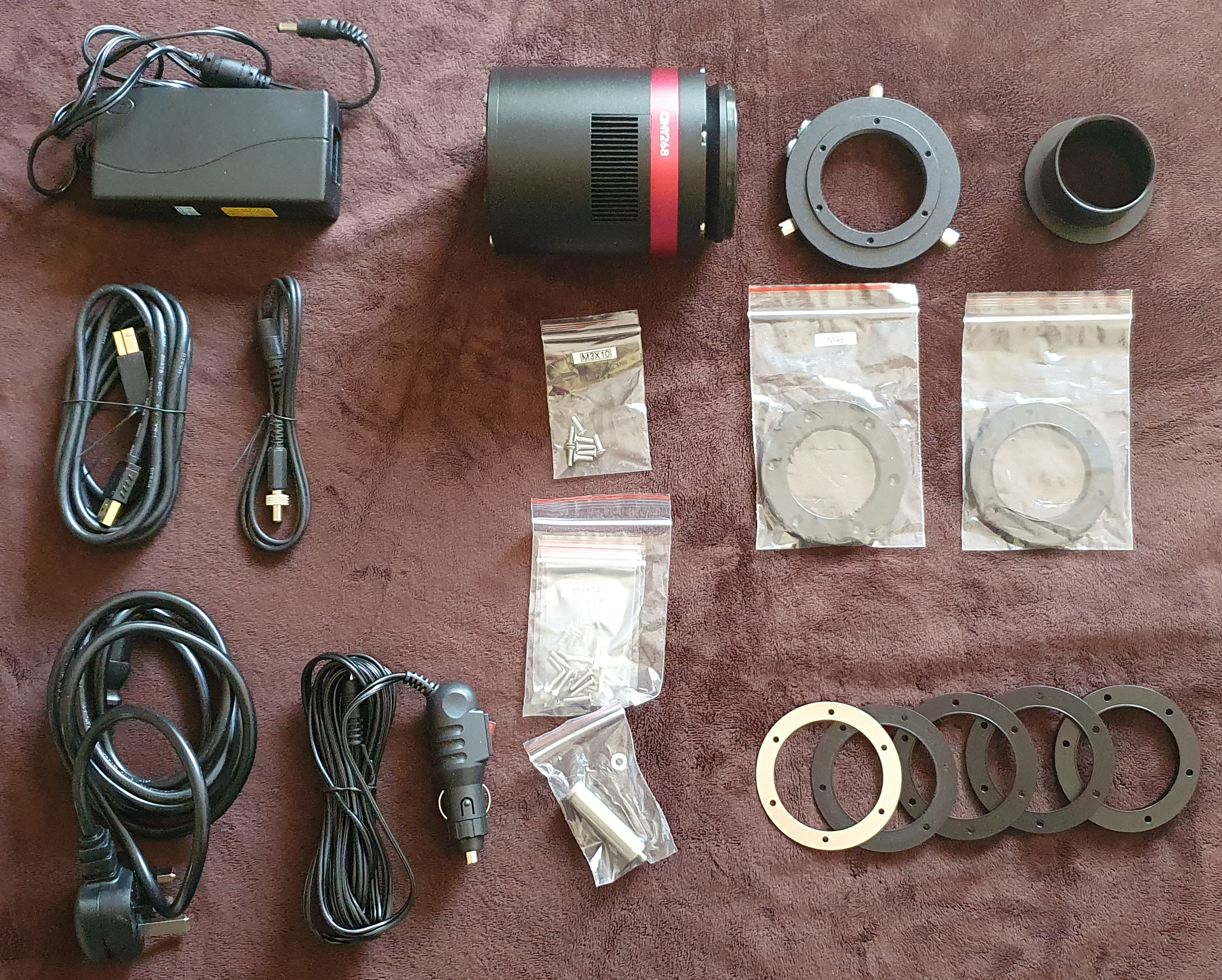
Opening the box I was greeted with a camera that was bigger and heavier than my 183M, but then the sensor is much bigger than the 183M anyway so this would be expected, but what I did not expect is the additional items that came with the camera:
Inside the box was:
QHY268C Photographic Version
UK mains plug for 12V AC adapter
12V AC adapter
Car 12v power cable
Self locking power cable
1.5M USB 3.0 cable
Dessicant drying tube
Self centering adapter plate
M54 to M48 adapter plate
M54 to 2″ nose adapter
A range of spacers to give you from 0.5mm to 13.5mm spacing
Associated screws for spacing adapters
QHY cameras have come along way since I bought my QHY183M, one of the things QHY has really worked on is amp glow, my early version of the QHY183M was renowned for was amp glow, which could be removed in image calibrations, but the QHY268C produces no amp glow whatsoever, below is a dark frame of 600S taken at -13.5C and you can clearly see there is no evidence of amp glow.
Single frame 600 seconds, Gain 26, Offset 30, -13.5C – Mono (Not Debayered)
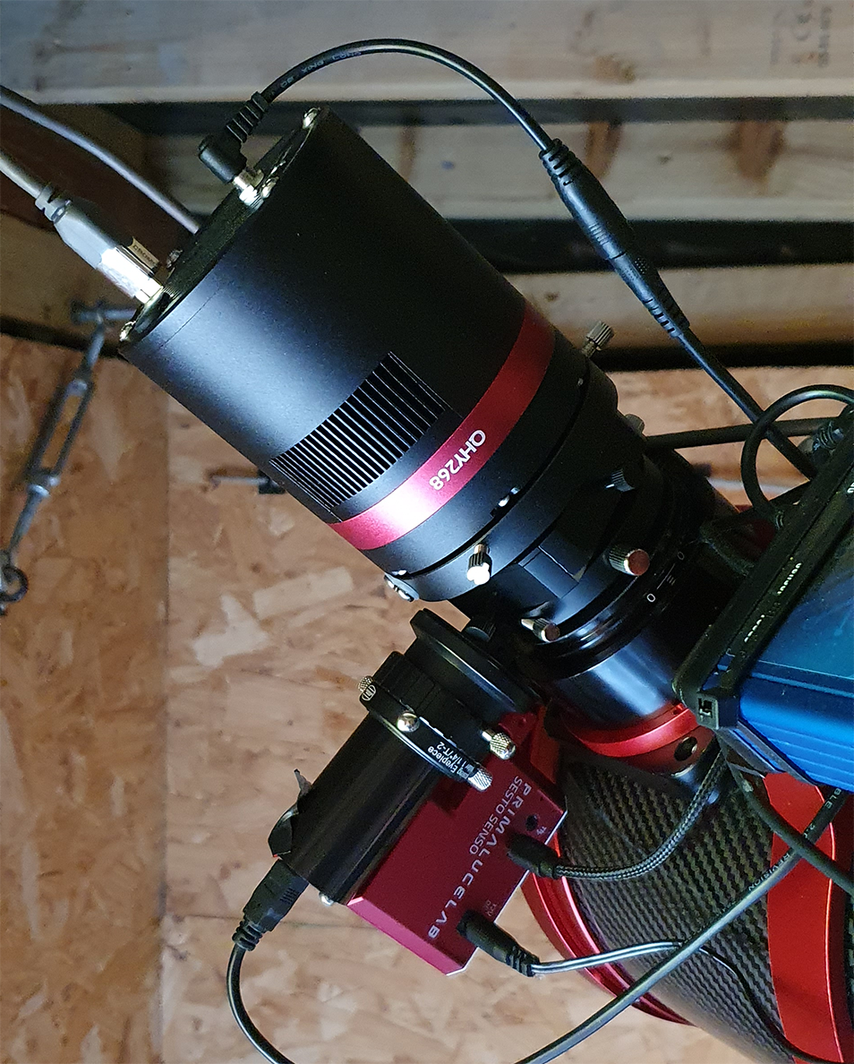
Attaching to the telescope was pretty straight forward as I had already planned the imaging train before the camera arrived, since I will be using the SharpStar 15028HNT F2.8 Paraboloid Astrograph which has an M48 thread, I decided to keep the whole imaging train at M48 except for the camera of course which has an M54 thread, so I did not actually need to use any of the adapters that came with the camera, the reason for this is because I wanted to include a filter drawer, so my image train consists of the following (from telescope to camera)
As you can see with all the above I reach my desired back focus of 55mm perfectly, if I was not going to be using a filter drawer (For my Optolong L-Pro and L-eXtreme filters), I would probably have stuck with the spacers that came with the camera. Below is a picture of the camera successfully connected to the telescope.
As far as settings go, after speaking with QHY on this at great length, I will be imaging in Mode 0 (Photographic mode) to avail of the massive 75ke full well, offset I will leave at 30, but Gain I will use two different settings, I will use Gain 0 for most bright objects with the L-Pro filter, but for the L-eXtreme, I’ll probably set a gain level of 26, luckily with SGPro I can set the gain level per object. From a cooling perspective I always image at -20C, one thing I have noticed is that this camera cools to exactly -35C below ambient, I tested this when the ambient temperature was 20.10 degrees, and the camera cooled down to -14.9C, it was always 25C lower until the ambient dropped below 15C and the camera remained at my setting of -20C.
The build quality of the camera is as expected having owned a QHY183M, one thing I did notice is that the fan in the QHY268C is much quieter than the 183M. Technical Details of the camera:
I can’t wait to get imaging with this camera, I have a very aggresive target list for this year in both RGB and Narrowband with the Optolong L-eXtreme filter, I will write part two of the review once I have some actual imaging data. Time to build my dark library.
After months of trying to get my trusty Sky-Watcher Quattro F4 to work with the ASA 0.73x reducer I decided to go all in on an F2.8 astrograph. After doing some research I stumbled across the SharpStar 15028HNT F2.8 Hyperboloid Newtonian Reflector from my local supplier 365Astronomy.
After toying with the idea and speaking to my good friend Nick from Altair Astro and with the idea of going back to a refractor, I decided that I could not go back to slower than F4 and I wanted something that in essence would work with a bigger sensor than my QHY183M, and the Sharpstar looked like it could work for me, so I placed my order with Zoltan from 365Astronomy and collected it the following day.
Unboxing the scope, I was like a young child at christmas, the scope came with a very sturdy protective hard case and removing the scope out of the case you could immediately feel that a lot of time and effort had gone into producing the 15028HNT.
With the scope unboxed I started to fit my equipment onto the scope. In order to fit my Sesto Senso I had to rotate the focuser 90 degrees clockwise due to the telescope mounting rings, this is when I noticed an isue that one of the grub screws on the focuser would not tighten and I needed to stop the backlash, fortunately there’s another grub screw on the other side that tightened and stopped the backlash.
Before I attached my imaging equipment, I had to ensure that the telescope was collimated, so I stumbled across the collimation guide which after speaking with my good friend Terry Hancock over at Grand Mesa Observatory who was also evaluating the same scope, we both agreed that the colimation guide wasn’t very well written as it mentioned nothing about collimating the primary. One thing that it mentioned is to remove the corrector, Sharpstar include a tool for you to remove the mounting plate and corrector, but here is a word of advice……..remove this when the telescope is cold, take that advice from someone who tried to remove it whilst it was warm!
I performed a laser collimation with my Concenter Eyepiece to check the secondary, and then a laser to check the primary, now the collimation guide says to remove the corrector, I have done validation with both the corrector removed and the corrector in place, and it made no difference whatsoever, so my opinion is to leave the corrector in place.
With the scope closely collimated, I mounted my StarlightXpress Filterwheel and Camera which with the 15028HNT is an M48 thread for the gear to screw onto.
I will post some images as soon as I have completed some, the weather has been pretty poor (probably because I bought a new scope), but the frames I have got so far are very sharp, pinpoint and I can honestly say I have never seen images come directly off the camera so sharp.
My field of view with the QHY183M is around 1.21 Arcsec/Pixel which gives me a FOV or around 1.81°x1.2° and I love the difraction spikes being at 45 degrees compared to the 90 degrees on the skywatcher and I already have a pretty full target list for this scope ready to go this season.
Apart from the couple of product issues I have experienced (Grub screw on focuser and tube clamp thumbscrew being threaded) I am extremely happy with the scope, it is performing really well and here are a couple of work in progress images that I have started
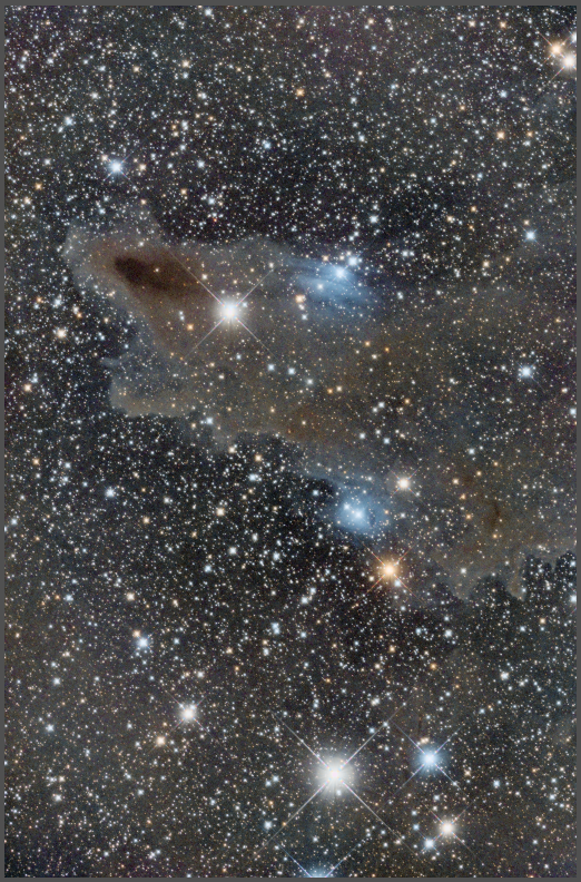
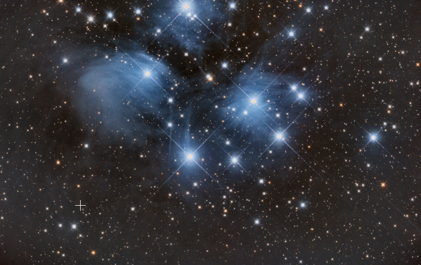
Dark Shark Nebula Moscaic Panel 1 – 51x300S in Red, 25x300S in Green and BlueElephant’s Trunk – 51x300S in 6nm HaM45 – Mosaic Panel 1 – 12x150S in R, G and B
After a few weeks, the telescope has held collimation very well, I have not had to perform any re-collimation, I will re-evaluate this in the much colder months of winter.
I am so happy with the scope that I am actually considering a second one for an OSC Camera with a bigger sensor.
M101 / NGC5457 or most commonly known as the Pinwheel Galaxy is a face on spiral galaxy in Ursa Major and has a distance of around 21 million light years from Earth.
The QHY183M picks up quite a lot of the Ha detail in this galaxy without me having to image separate Ha Filter data
Image Details:
101x150S in R
101x150S in G
101x150S in B
Total Capture time: 12.6 Hours
Acquisition Dates: Feb. 27, 2019, March 29, 2019, March 30, 2019, April 1, 2019, April 11, 2019, April 12, 2019, April 14, 2019
All frames had 101 Darks and Flats applied
Equipment Details:
Imaging Camera: Qhyccd 183M Mono ColdMOS Camera at -20C
Imaging Scope: Sky-Watcher Quattro 8″ F4 Imaging Newtonian
Guide Camera: Qhyccd QHY5L-II
Guide Scope: Sky-Watcher Finder Scope
Mount: Sky-Watcher EQ8 Pro
Focuser: Primalucelab ROBO Focuser
FIlterwheel: Starlight Xpress Ltd 7x36mm EFW
Filters: Baader Planetarium RGB
Power and USB Control: Pegasus Astro USB Ultimate Hub Pro
Acquisition Software: Main-Sequence Software Inc. Sequence Generator Pro
Processing Software: PixInsight 1.8.6
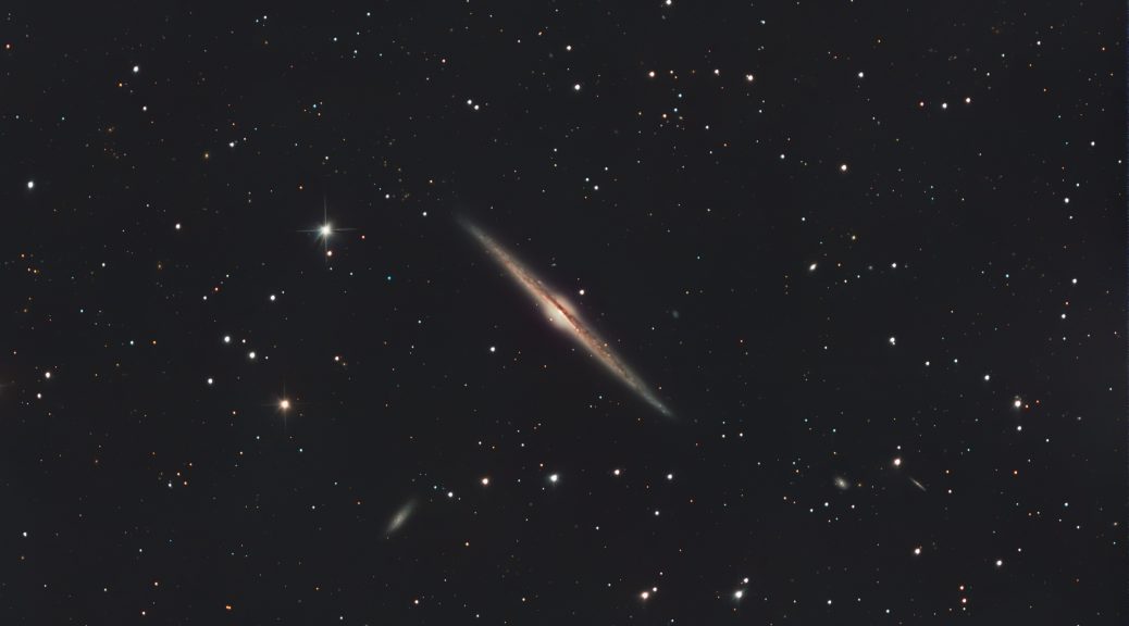
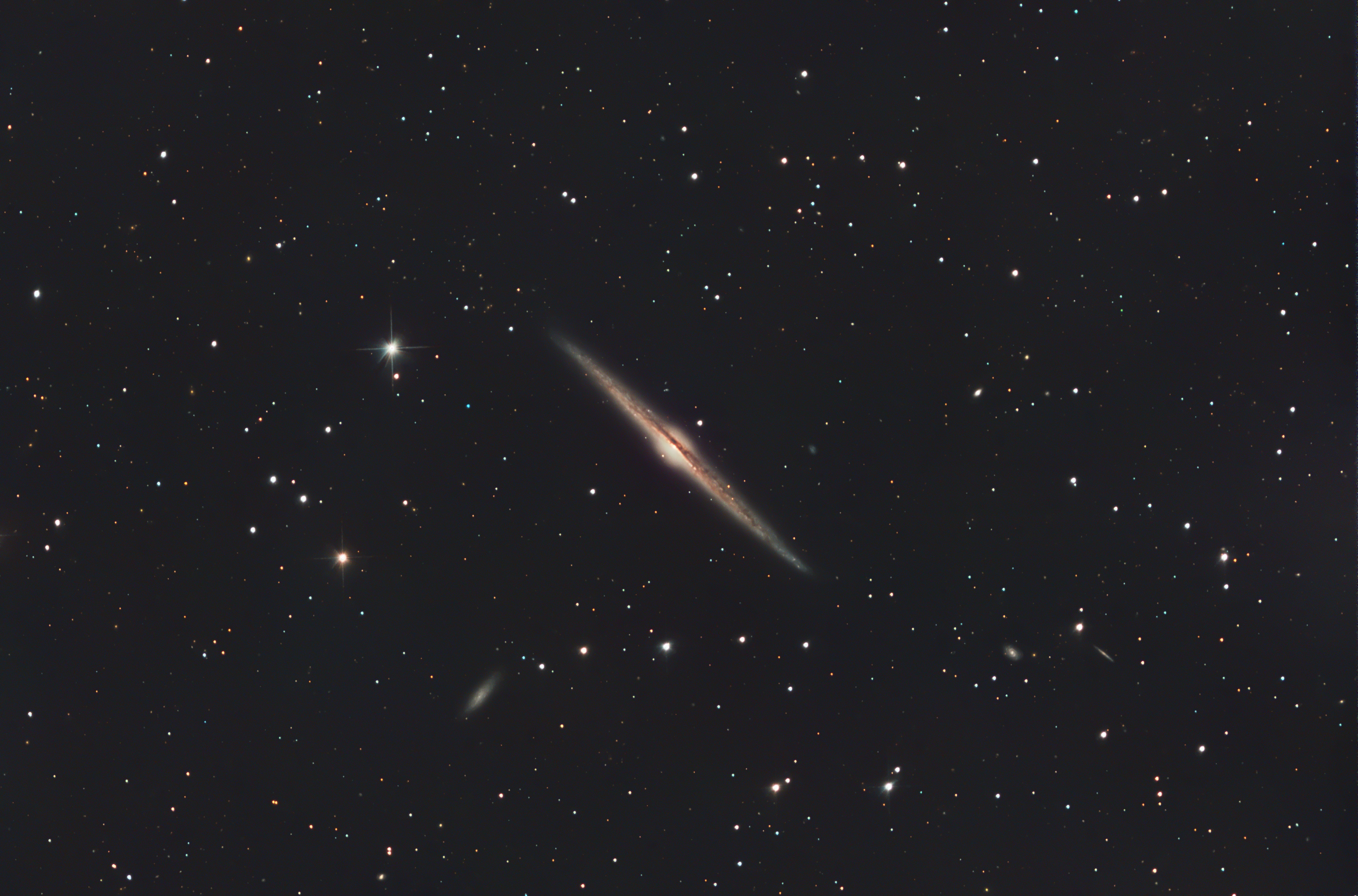
The Needle Galaxy is located int he constellation of Coma Berencies and is an edge on spiral galaxy at a distance of 30-50 million light years from earth
Image Details:
101x150S in R
101x150S in G
101x150S in B
Total Capture time: 12.6 Hours
Acquisition Dates: Jan. 28, 2019, Feb. 3, 2019, Feb. 25, 2019, Feb. 26, 2019, Feb. 27, 2019, March 26, 2019, March 29, 2019, March 30, 2019, April 1, 2019
Equipment Details:
Imaging Camera: Qhyccd 183M Mono ColdMOS Camera at -20C
Imaging Scope: Sky-Watcher Quattro 8″ F4 Imaging Newtonian
Guide Camera: Qhyccd QHY5L-II
Guide Scope: Sky-Watcher Finder Scope
Mount: Sky-Watcher EQ8 Pro
Focuser: Primalucelab ROBO Focuser
FIlterwheel: Starlight Xpress Ltd 7x36mm EFW
Filters: Baader Planetarium RGB
Power and USB Control: Pegasus Astro USB Ultimate Hub Pro
Acquisition Software: Main-Sequence Software Inc. Sequence Generator Pro
Processing Software: PixInsight 1.8.6
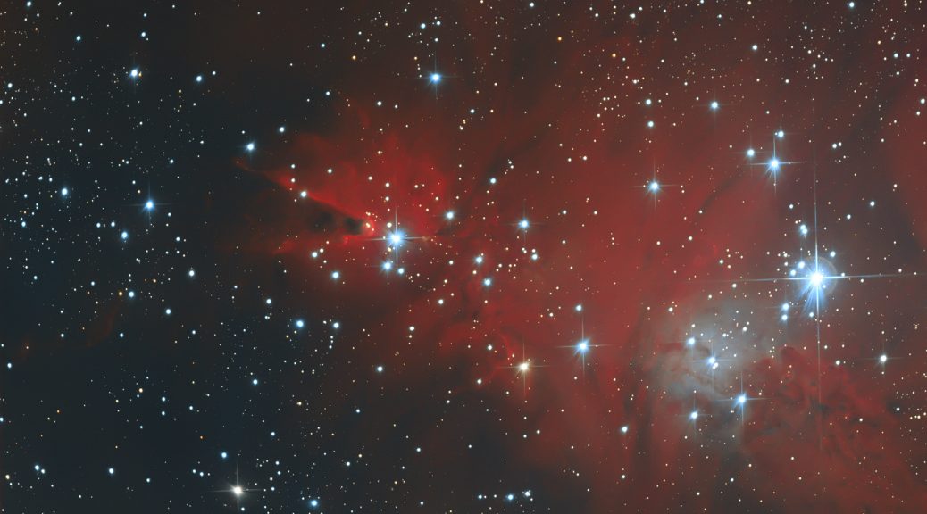
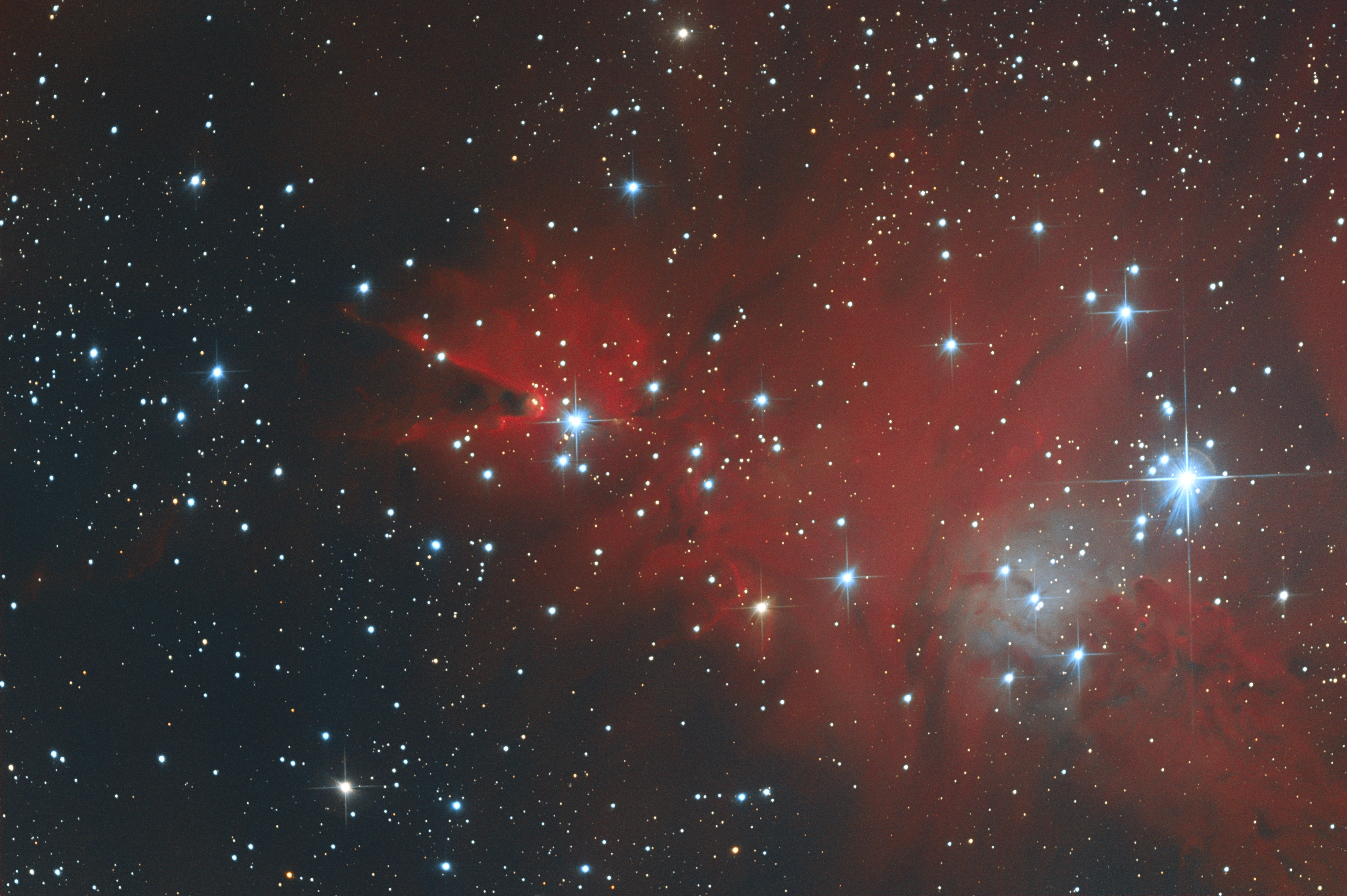
Located in the constellation of Moneceros, this image shows both the Cone Nebula and the Christmas Tree Cluster, located around 2600 light years from earth the Cone Nebula being an emmision Nebula
Image Details:
101x150S in R
101x150S in G
101x150S in B
101x300S in Ha
Total capture time: 21 Hours
Acquisition Dates: Jan. 9, 2019, Jan. 31, 2019, Feb. 3, 2019, Feb. 14, 2019, Feb. 15, 2019, Feb. 23, 2019, Feb. 24, 2019, Feb. 25, 2019, Feb. 26, 2019, Feb. 27, 2019, Feb. 28, 2019, March 24, 2019, March 25, 2019, March 26, 2019, March 28, 2019, March 29, 2019
The NBRGB Script in PixInsight was used to blend the Ha into the RGB Image
101 Darks, Flats and Flat Darks were used in the frame calibration
Equipment Details:
Imaging Camera: Qhyccd 183M Mono ColdMOS Camera at -20C
Imaging Scope: Sky-Watcher Quattro 8″ F4 Imaging Newtonian
Guide Camera: Qhyccd QHY5L-II
Guide Scope: Sky-Watcher Finder Scope
Mount: Sky-Watcher EQ8 Pro
Focuser: Primalucelab ROBO Focuser
Filterwheel: Starlight Xpress Ltd 7x36mm EFW
Filters: Baader Planetarium RGB and Ha
Power and USB Control: Pegasus Astro USB Ultimate Hub Pro
Acquisition Software: Main-Sequence Software Inc. Sequence Generator Pro
Processing Software: PixInsight 1.8.6